Math4225 Answer to Homework 2

2.4.2 (1) If d_∞(f, g) < ε and max_0≤t≤1 f = f(t₀), then g(t₀) > f(t₀) - ε, so that M(g) > M(f) - ε. Switching the roles of f and g, we also have M(f) > M(g) - ε. Therefore |M(f) - M(g)| < ε. This shows that M is continuous with respect to the L_∞-metric.

On the other hand, M is not continuous with respect to the L₁-metric. This can be seen easily by constructing g so that has the area between f and g is very small area, but g is significantly bigger than max_0≤t≤1 f somewhere.

By d₁ ≤ d_∞, we have |I(f) - I(g)| ≤ d₁(f, g) ≤ d_∞(f, g). Therefore d_∞(f, g) < ε implies |I(f) - I(g)| < ε. This implies that I is continuous with respect to the L_∞-metric.

(3) Take the metric on X x Y to be d((x, y), (x', y')) = d_X(x, x') + d_Y(y, y').

For the L_∞-metric, we have d_∞(σ(f + g), σ(f' + g')) = max_0≤t≤1 |f(t) + g(t) - f'(t) - g'(t)| ≤ max_0≤t≤1|f(t) - f'(t)| + max_0≤t≤1|g(t) - g'(t)| = d_∞(f, g) + d_∞(f', g') = d_∞((f, f'), (g, g')), where the right side is the product L_∞-metric on C[0, 1]². The inequality shows that σ is continuous with respect to the L_∞-metric.

For the L_∞-metric, we have d₁(σ(f + g), σ(f' + g')) = ∫|f(t) + g(t) - f'(t) - g'(t)|dt ≤ ∫|f(t) - f'(t)|dt + ∫|g(t) - g'(t)|dt = d₁(f, g) + d₁(f', g') = d₁((f, f'), (g, g')), where the right side is the product L₁-metric on C[0, 1]². The inequality shows that σ is continuous with respect to the L₁-metric.

2.4.3 By d₁ ≤ d_∞, we have d₁(id(f), id(g)) ≤ d_∞(f, g). This implies that the identity map is continuous from the L_∞-metric to the L₁-metric. The converse is not true because we could have very small d₁(f, g) and very big d_∞(f, g) at the same time.

2.4.4 Let (x₀, y₀) be rational numbers and ε > 0. The subsequent argument will be for the case both x₀ and y₀ are nonzero. The case at least one of them is zero is simpler and will be omitted.

Since both x₀ and y₀ are nonzero, we may write x₀ = (m₀/n₀)p^a₀ and y₀ = (k₀/l₀)p^b₀ in the usual way. Then we assume x - x₀ = (m/n)p^a and y - y₀ = (k/l)p^b in the usual way, with d_p-adic(x, x₀) = p^-a < δ and d_p-adic(y, y₀) = p^-b < δ, where δ > 0 is to be determined. Our goal is to determine δ so that d_p-adic(xy, x₀y₀) < ε. Note that

xy - x₀y₀
= (x - x₀)[(y - y₀) + y₀] + x₀(y - y₀)
= (m/n)p^a[(k/l)p^b + (k₀/l₀)p^b₀] + (m₀/n₀)p^a₀(k/l)p^b
= [(m/n)p^a+b-c + (mk₀/nl₀)p^a+b₀-c + (m₀k/n₀l)p^a₀+b-c]p^c,

where c = min{a + b₀, a + b, a₀ + b}. The sum in the bracket is of the form (r/s)p^d, where r and s are integers not divisible by p, and d is a non-negative integer. Thus we have d_p-adic(xy, x₀y₀) = p^-c-d ≤ p^-c. The problem is now reduced to the choice of δ so that p^-a < δ and p^-b < δ implies p^-c < ε. Since this is equivalent to p^-a₀δ ≤ ε, p^-b₀δ ≤ ε, δ² ≤ ε, we should choose d = min{p^a₀ε, p^b₀ε, √ε}.

2.4.5 By A ∪ E - B ∪ E ⊂ A - B and B ∪ E - A ∪ E ⊂ B - A, we have (A ∪ E - B ∪ E) ∪ (B ∪ E - A ∪ E) ⊂ (A - B)∪(B - A). By taking minimum (note: X ⊂ Y ⇒ minX ≥ minY) and reciprocal, we conclude that d(A ∪ E, B ∪ E) ≤ d(A,B). Then it follows from Exercise 2.4.8 that union with E is a continuous map.

We also have A ∩ E - B ∩ E ⊂ A - B. Then by the similar argument as before, we may prove d(A ∩ E, B ∩ E) ≤ d(A,B), which implies that intersection with E is a continuous map.

Finally, substracting E is the same as intersecting N - E. Therefore the substraction is also continuous.

2.4.6 For a ∈ X and ε > 0, we need to find δ > 0, such that d(x, a) < δ implies |f(x) + g(x) - f(a) - g(a)| < ε.

Note that in order for the final conclusion to hold, it suffices to have |f(x) - f(a)| < ε/2 and |g(x) - g(a)| < ε/2. Based on this observation, we come up with the following argument: For the given a and ε, by the continuity of f, we have δ₁ > 0, such that d(x, a) < δ₁ implies |f(x) - f(a)| < ε/2. Similarly, by the continuity of g, we have δ₂ > 0, such that d(x, a) < δ₂ implies |g(x) - g(a)| < ε/2. Choose δ = min{δ₁,δ₂}. Then d(x, a)< δ implies

|f(x) + g(x) - f(a) - g(a)| ≤ |f(x) - f(a)| + |g(x) - g(a)| < ε/2 + ε/2 = ε.

Now let us prove the continuity of fg. The conclusion we would like to reach is |f(x)g(x) - f(a)g(a)| < ε. The key observation is the inequality

|f(x)g(x) - f(a)g(a)|
= |f(x)g(x) - f(a)g(x) + f(a)g(x) - f(a)g(a)|
≤ |f(x) - f(a)| |g(x)| + |f(a)| |g(x) - g(a)|.

Based on the analysis above, we come up with the following argument: For the given a and ε, we will postulate a small number ε' > 0, which will depend only on the given data (f, g, a, ε) and will be determined at the end. By the continuity of f, we have δ₁ > 0, such that d(x, a) < δ₁ implies |f(x) - f(a)|< ε'. Similarly, by the continuity of g, we have δ₂ > 0, such that d(x, a)< δ₂ implies |g(x) - g(a)| < ε'. Choose δ = min{δ₁,δ₂}. Then d(x, a) < δ implies

|f(x)g(x) - f(a)g(a)|
≤ |f(x) - f(a)| |g(x)| + |f(a)| |g(x) - g(a)|
< ε'(|g(x) - g(a)| + |g(a)|) + |f(a)|ε'
< ε'(ε' + |g(a)|) + |f(a)|ε',

which will be ε as long as ε' satisfies

ε'² + |g(a)|ε' + |f(a)|ε' < ε.

This suggests us that we could use ε' = (1 + |f(a)| + |g(a)|)^-1 at the beginning of our arguement.

2.4.8 For any a ∈ X and ε > 0, we take δ = ε/c. Then d_X(x, a) < δ implies d_Y(f(x), f(a)) < c d_X(x, a) < c δ = ε.

2.4.10 For any b ∈ X (I choose b because a has been used) and ε > 0, we take δ = ε. Then d(x, b) < δ implies |f(x) - f(b)| = |d(x, a) - d(b, a)| ≤ d(x, b) < ε, where ≤ follows from Exercise 2.1.6.

2.4.11 For any (a, b) ∈ X×X and ε > 0, we take δ = ε/2. Then d((x, y), (a, b)) < δ implies d(x, a) < δ and d(y, b) < δ. Then it follows from Exercise 2.1.6 that |d(x, y) - d(a, b)| ≤ |d(x, a)| + |d(y, b)| < 2δ = ε.

2.4.12 Suppose f is continuous and lim a_n = x. For this x and any ε > 0, there is δ > 0, such that

d(y, x) < δ ⇒ d(f(y), f(x)) < ε.

By lim a_n = x, for this δ > 0, there is N, such that

n > N ⇒ d(a_n, x) < ε.

Combining thwe two implicaitons together, we get

n > N ⇒ d(f(a_n), f(x)) < ε.

This proves that lim f(a_n) = f(x).

On the other hand, if f is not continuous, then there is x and ε > 0, such that for any δ > 0, there is a satisfying d(a, x) < δ, yet d(f(a), f(x)) ≥ ε. By choosing δ = 1/n, we get a_n satisfying d(a_n, x) < 1/n, yet d(f(a_n), f(x)) ≥ ε. Therefore we have lim a_n = x, yet lim f(a_n) ≠ f(x). This proves the other direction.

2.4.14 If Y has the discrete metric, then the continuity of f: X → Y means that f^-1(U) is open for any subset U of Y. This is often not true. For a concrete example, we consider

f(x) = x: (R, usual metric) → (R, discrete metric)

The subset U = {0} is open in (R, discrete metric). However, f^-1(U) = U is not open in (R, usual metric). Therefore f is not continuous.

2.4.15 Denote f(x) = d(x, A). The following picture suggests that |f(x) - f(y)| ≤ d(x, y).

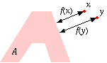
To rigorously prove |f(x) - f(y)| ≤ d(x, y), we note that we have

f(y) ≤ d(y, a) ≤ d(x, a) + d(x, y),

for any a ∈ A, where the first ≤ comes from the definition of f(y), and the second ≤ comes from triangle inequality. Since the left side of the inequality is independent of a, we we take the inf of the right side for all a ∈ A, and get

f(y) ≤ f(x) + d(x, y).

By exchanging the roles of x and y, we can similarly prove

f(x) ≤ f(y) + d(x, y).

Thus we conclude that |f(x) - f(y)| ≤ d(x, y).

The inequality implies the continuity of f at y ∈ X in the following way: For any y ∈ X and ε > 0, we choose δ = ε. Then we have

d(x, y) < δ ⇒ |f(x) - f(y)| ≤ d(x, y) < δ = ε,

which verifies the definition of the continuity.

Finally, we have

A^ε = {x ∈ X: d(x, a)< ε for some a ∈ A} = {x ∈ X: f(x) < ε} = f^-1(-∞,ε).

Since f is continuous and (-∞,ε) is open, we conclude that A^ε is open.

2.5.1

Exercise 2.3.5

(1) The limit points in L_∞-metric are f satisfying f(0) ≥ 0. The limit points in L₁-metric are all functions.

(2) The limit points in L_∞-metric are f satisfying f(0) ≥ 0. The limit points in L₁-metric are all functions.

(3) The limit points in L_∞-metric are f satisfying f(0) ≥ f(1). The limit points in L₁-metric are all functions.

(4) The limit points in L_∞-metric are f satisfying t + 1 ≥ f(t) ≥ t². The limit points in L₁-metric are the same.

(5) The limit points in L_∞-metric are f satisfying t + 1 ≥ f(t) ≥ t². The limit points in L₁-metric are the same.

(6) The limit points in L_∞-metric are f satisfying ∫₀¹f(t)dt ≥ 0. The limit points in L₁-metric are the same.

(7) The limit points in L_∞-metric are f satisfying ∫₀¹f(t)dt ≥ 0. The limit points in L₁-metric are the same.

(8) The limit points in L_∞-metric are f satisfying ∫₀^1/2f(t)dt ≥ ∫_1/2¹f(t)dt. The limit points in L₁-metric are the same.

Exercise 2.3.6 Note that the 2-adic metric is an ultrametric: d(x, y) ≤ max{d(x, z), d(z, y)}.

(1) Suppose x ≠ 0 is a limit of integers. By the ultrametric property, d(x, 0) ≤ max{d(x, n), d(n, 0)}. By chosing integer n so that d(x, n) < ε = d(x, 0), we find d(x, 0) ≤ d(n, 0) ≤ 1. Therefore the denominator of x is an odd number.

Conversely, suppose b is an odd number such that there is an integer k ≥ 1 satisfying 2^k = 1 modulo b. Then we get 2^kn = 1 + bm for any n and some integer m. This implies 2^kn/b = 1/b + m, so that d(1/b, m) = 2^-kn can be as small as possible. This proves that 1/b is a limit point of all integers.

Now we claim that any odd number b has the property. The reason comes from the group theory. Since the number 2 is coprime to b, it is an invertible element in the group (Z/bZ)^* of multiplicatively invertible elements in the ring Z/bZ. The group is finite with order k (actually denoted φ(b) and called the Euler function). From theory of finite groups, 2^k is the identity element in the group (Z/bZ)^*, which means 2^k = 1 modulo b.

It is not difficult to prove that if x and y are limit points of integers, then x + y and -x are also limit points. Therefore if 1/b is a limit point, then a/b is also a limit point. In particular, by taking a to be multiples of b, integers are limit points. We conclude that the limit points are those with odd numbers as denominator (including 1 as denominator).

(2) The set is obtained by multiplying 2 to all the points in the set in (1). By d(2x, 2y) = d(x, y)/2, it is easy to see that the limit points are obtained by multiplying 2 to the limit points in (1). In other words, the limit points are of the form even/odd.

(3) Suppose x ≠ 0 is a limit of odd/even. By the ultrametric property, d(r, 0) ≤ max{d(r, x), d(x, 0)}. By chosing r = odd/even so that d(x, r) < ε = d(x, 0), we find d(x, 0) ≥ d(r, 0) ≥ 2. Therefore x is also of the form odd/even.

Conversely, assume x is of the form = odd/even. Then x + 2^k is also of the form = odd/even and d(x, x + 2^k) = 2^-k. This shows that x is a limit point.

(4) Suppose x ≠ 0 is a limit of even/odd. By the ultrametric property, d(x, 0) ≤ max{d(x, r), d(r, 0)}. By chosing r = even/odd so that d(x, r) < ε = d(x, 0), we find d(x, 0) ≤ d(r, 0) ≤ 1/2. Therefore x is also of the form even/odd.

Conversely, assume x is of the form = even/odd. Then x + 2^k is also of the form = even/odd and d(x, x + 2^k) = 2^-k. This shows that x is a limit point.

(5) By an argument similar to (3), a limit point must has odd numerator. Conversely, assume x = a/b, with a odd. Then for any k, a is a generator in the cyclic additive group Z/2^kZ. This implies that na = b modulo 2^k for some integer n. Dividing nb, we get x - 1/n = 2^km/n. If k is bigger than the number of 2-factors in b, then the number of 2-factors in n must be the same as the number in b. Therefore the number of 2-factors in 2^km/n is getting bigger as k gets bigger. In other words, d(x, 1/n) can become as small as we want. We conclude that the limit points are those with odd numerator.

(6) For any rational number x = a/b, we have x - x/(2ⁿ+1) = a2ⁿ/b(2ⁿ+1). This implies that d(x, x/(2ⁿ+1)) can become as small as we want as n gets bigger. Since x/(2ⁿ+1) has small absolute value as n gets bigger, we conclude that any rational number is a limit.

Exercise 2.3.7

(1) All subsets with numbers bigger than 10.

(2) No limit points.

(3) All subsets of even numbers.

(4) All subsets that does not contain 100.

(5) All subsets.

(6) All single subsets and empty set.

2.5.2 Suppose x ∉ A is a limit point of A. Then there is a ∈ A, such that d(a, x) < ε/2. If there is another b ∈ A that also satisfies d(b, x) < ε/2. Then d(a, b) < ε, contradicting to the assumption about the distance between the elements of A. Therefore a is the only element of A satisfying d(a, x) < ε/2. Then for δ = d(a, x) > 0 (x ≠ a because x ∉ A), there is no b ∈ A satisfying d(b, x) < δ. This shows that x is not a limit point of A.

Now consider x ∈ A. Then by the assumption, there is no a ∈ A satisfying a ≠ x and d(a, x) < ε. Therefore x is not a limit point of A.

2.5.3 Let d'(x, y) < c d(x, y). Then B_d(x, ε) ⊂ B_d'(x, cε), which implies (A - x) ∩ B_d(x, ε) ⊂ (A - x) ∩ B_d'(x, cε). Therefore (A - x) ∩ B_d(x, ε) is nonempty for arbitrary ε > 0 implies (A - x) ∩ B_d'(x, cε) is nonempty for arbitrary ε > 0 (ε is arbitrary is equivalent to cε is arbitrary). In other words, the limit points of A in metric d must be limit points of A in metric d'.

2.5.4 1. (A - x) ∩ B_d(x, ε) ≠ ∅ implies (B - x) ∩ B_d(x, ε) ≠ ∅.

2. Since A and B are contained in A ∪ B, by part 1 we conclude that A' ∪ B' ⊂ (A ∪ B)'.

To prove the inclusion in another direction, we assume x is not in A' ∪ B'. Then we have (A - x) ∩ B_d(x, ε) = ∅ and (B - x) ∩ B_d(x, ε') = ∅ for some ε, ε' > 0. This implies (A ∪ B - x) ∩ B_d(x, min{ε, ε'}) ⊂ ((A - x) ∩ B_d(x, ε)) ∪ ((B - x) ∩ B_d(x, ε')) = ∅. Therefore x is not in (A ∪ B)'.

The following argument for (A ∪ B)' to be contained in A' ∪ B' is wrong:

Let x be a limit point of A ∪ B. Then (A ∪ B - x) ∩ B_d(x, ε) ≠ ∅ for any ε > 0. Since (A ∪ B - x) ∩ B_d(x, ε) = ((A - x) ∩ B_d(x, ε)) ∪ ((B - x) ∩ B_d(x, ε)), we have (A - x) ∩ B_d(x, ε) ≠ ∅ ot (B - x) ∩ B_d(x, ε) ≠ ∅.

The subtle point is that the reasoning here only shows that for ONE ε, we find one a in A (or in B). It does not exclude the possibility that for ANOTHER ε, we find b in B instead of A. On the other hand, we are required to make up our mind on whether x is a limit point of A or not BRFORE the choice of ε. In other words, we cannot change our mind for different choices of ε.

3. By part 1 it is easy to see that (A ∩ B)' ⊂ A' ∩ B'. However, the containment other way around is not true.

Consider X = R with the usual metric. Take A = (-1, 0), B = (0, 1). Then A ∩ B is empty and so is (A ∩ B)'. On the other hand, A' ∩ B' = [-1, 0] ∩ [0, 1] = {0} is not empty.

4. Let x ∈ A''. Then for any ε > 0, we have a', such that

1) a' ∈ A', 2) a' ≠ x, 3) d(a', x) < ε.

Since a' ∈ A', for ε' = min{d(a', x), ε - d(a', x)} > 0, we have a, such that

1) a ∈ A, 2) a ≠ a', 3) d(a, a') < ε'.

Then d(a, a') < ε' ≤ d(a', x) implies a ≠ x. Moreover, we have

d(a, x) ≤ d(a', x) + d(a, a') < d(a', x) + ε' ≤ d(a', x) + (ε - d(a', x)) = ε.

Thus we conclude that

1) a ∈ A, 2) a ≠ x, 3) d(a, x) < ε,

and x ∈ A'.

2.5.5 Suppose there is such a sequence. Since a_i ≠ a_j for i ≠ j, we have at most one a_n equal to x. By deleting this a_n if necessary, we may assume all a_n ≠ x. Now for any ε > 0, we have some a_n, such that d(a_n, x) < ε. Thus we have

1) a_n ∈ A, 2) a_n ≠ x, 3) d(a_n, x) < ε.

This shows that x is a limit point of A.

Conversely, assume x is a limit point of A. Then we can find a sequence of points as follows

1) a₁ ∈ A, 2) a₁ ≠ x, 3) d(a₁, x) < 1,

2) a₂ ∈ A, 2) a₂ ≠ x, 3) d(a₂, x) < min{d(a₁, x), 1/2},

3) a₃ ∈ A, 2) a₃ ≠ x, 3) d(a₃, x) < min{d(a₂, x), 1/3},

…

n) a_n ∈ A, 2) a_n ≠ x, 3) d(a_n, x) < min{d(a_n-1, x), 1/n},

…

This sequence {a_n} is a non-repetitive sequence in A with lim_n→∞d(a_n, x) = 0.

2.5.8 Since x ∈ U and U is open, we have B(x, δ) ⊂ U for some δ > 0. Now for any ε satisfying δ ≥ ε > 0, since x is a limit point of A, the intersection (A - x) ∩ B(x, ε) ≠ ∅. By B(x, ε) ⊂ B(x, δ) ⊂ U, this implies (A ∩ U - x) ∩ B(x, ε) = (A - x) ∩ U ∩ B(x, ε) = (A - x) ∩ B(x, ε) ≠ ∅.

We have proved (A ∩ U - x) ∩ B(x, ε) ≠ ∅ for any δ ≥ ε > 0. Now for ε ≥ δ, (A ∩ U - x) ∩ B(x, ε) is even bigger and should still be nonempty. Thus we have shown x is a limit point of A ∩ U.

The fact that A ∩ U is infinite follows from Exercise 2.5.2 and the existence of limit points for A ∩ U.

2.5.9 Not true. If f is a constant map, then f(A) conatined only one point and has no limit points.

2.5.10 We clearly have d(x, A) = 0 for x ∈ A. On the other hand, let x be a limit point of A. Then for any ε > 0, there is a, such that

1) a ∈ A, 2) a ≠ x, 3) d(a, x) < ε.

In particular, we have d(x, A) ≤ d(a, x) < ε. Since ε can be arbitarily small, and d(x, A) does not depend on ε, we conclude that d(x, A) = 0.

Conversely, we need to show that d(x, A) = 0 and a ∉ A implies a is a limit point of A. Since d(x, A) = 0, for any ε > 0, we can find a ∈ A, such that d(a, x) < ε. Thus the first and the third conditions are satisfied. Moreover, since a ∈ A and x ∉ A, we have a ≠ x. Thus the second condition is also satisfied. In conclusion, x is a limit point of A.

2.6.1 In discrete topology, any subset is open and closed. In R_usual, (0, 1) is open but not closed, [0, 1] is closed but not open, and [0, 1) is neither closed nor open.

Let A be an open subset of R_usual, and A ≠ ∅ or R. Then A is a nonempty disjoint union of open intervals. Let (a, b) be one such open interval. Then one of a, b must be finite (because (a, b) cannot be the whole R), and this one is not in A. Without loss of generality, we may assume a is finite and not in A. Then a is a limit point of (a, b), which implies a is a limit point of A. Since a ∉ A, we see that A is not closed.

2.6.2 By Exercise 2.5.3, if d'(x, y) < c d(x, y), then d'-closed implies d-closed.

2.6.3 By Exercise 2.5.10, A is closed if and only if d(x, A) = 0 implies x ∈ A.

2.6.5 Let x be a limit point of a ball B(a, ε) in an ultrametric space. Then for any δ > 0, the intersection (B(a, ε) - x) ∩ B(x, δ) ≠ ∅. Let y be a point in the intersection. Then by y ∈ B(a, ε) and Exercise 2.19, B(a, ε) = B(y, ε). Moreover, by y ∈ B(x, δ) and Exercise 2.19, B(x, δ) = B(y, δ). By choosing δ = ε, we conclude that x ∈ B(x, δ) = B(y, δ) = B(y, ε) = B(a, ε). Thus we have proved that B(a, ε) contains all its limit points.

Alternative proof: We prove that the complement X - B(a, ε) is open. Suppose x ∉ B(a, ε). Then we claim that B(x, ε) ∩ B(a, ε) = ∅. The claim would imply that B(x, ε) is still contained in X - B(a, ε), and the openness of X - B(a, ε) follows by definition.

Suppose B(x, ε) ∩ B(a, ε) ≠ ∅. Let y be in the intersection. Then by y ∈ B(x, ε) and Exercise 2.19, B(x, ε) = B(y, ε). Moreover, by y ∈ B(a, ε) and Exercise 2.19, B(a, ε)= B(y, ε). Therefore B(x, ε) = B(y, ε) = B(a, ε). This implies x ∈ B(a, ε), contradicting to original assumption.

2.6.6 If x is a limit point of the closed ball, then for any δ > 0, there is y in the closed ball, such that d(x, y) < δ. Since y in the closed ball, we have d(y, a) ≤ ε. Therefore d(x, a) < δ + ε for any δ > 0. This implies d(y, a) ≤ ε. In other words, x is also in the closed ball.

2.6.7 If A contains all the limits of convergent sequences in A, then by Exercise 2.5.5, A contains all its limt points and is therefore closed. Conversely, suppose A is closed and a_n ∈ A is a sequence converging to x. Then either a_n are distinct for sufficiently big n, or there is a constant subsequence. In the first case, the limit x is, by Exercise 2.5.5, a limit point of A. Since A is closed, we get x ∈ A. In the second case, the constant sequence is the same as the limit point x repeating itself again and again. Since the subsequence lies in A, we get x ∈ A.

2.6.8 [1/n, 1] is closed. But ∪_n [1/n, 1] = (0, 1] is not closed.

2.6.9 1. Not closed: 0 is a limit point of (0, 1] in A. But 0 is not contained in (0,1].

2. Closed: The trouble point 0 in the prwvious example is no longer included in B. Once may either see the closedness by considering the limit points of (0, 1] in B (which is (0, 1] itself). Or one can use the fact that the complement (1, ∞) is open in B.

3. Not closed: The trouble is the same as in 1.

4. Closed: The whole space is always closed.

5. Not closed: Same trouble as in 1.

6. Closed: Same reason as in 2.

2.6.10 A subset A has limit point x if and only if A is infinite and x = 0. Therefore the closed subsets are the finite subsets and the infinite subsets that contain 0.

2.6.11 1. closed: It is the product of closed subsets {0} and (-∞, 5] (see Exercise 2.6.15)

2. closed: It is the product of closed subsets {positive integers} and {integers} (see Exercise 2.6.3)

3. not closed: (0,1) is a limit point but is not in the subset.

4. closed: It is the preimage of the single point {0} under the continuous map y - x²: R² → R.

2.6.12 1. The map f(x, y, z) = x³ - y³ + 2z² - xy - 2yz + 3zx: R³_usual → R_usual is continuous. The subset is f^-1[-1, 3].

2. The map f(x, y, z, w) = (x⁴ + y⁴ - z⁴ - w⁴, x³ + y³ - z³ - w³): R⁴_usual → R²_usual is continuous. The subset is f^-1(0,0), the preimage of the single origin point.

3. The map F(M) = M^tM: Matrix(n×n) → Matrix(n×n) is continuous (for n = 2, write F explicitly as a map from R⁴ to R⁴ and convince yourself that F is continuous). The subset is F^-1(I), the preimage of the identity matrix.

4. The characteristic polynomial F(M) = det(tI - M): Matrix(n×n) → P_n is a continuous map, where the space P_n of degree n polynomials may be identified with Rⁿ⁺¹. The subset is F^-1((t - 1)ⁿ), the preimage of the single polynomial (t - 1)ⁿ.

2.6.13 In a square matrix M = (a_ij)_1≤i,j≤n, the k-th principal submatrix M(k) = (a_ij)_1≤i,j≤k is formed by the entries in row 1 through k and columns 1 through k. The coefficients in a quadratic form form a symmetric matrix M. The quadratic form is semi-positive definite if and only if in the corresponding symmetric matrix, the determinants of all principal submatrices are non-negative. In other words, the semi-positive definite symmetric matrices are exactly F^-1( [0, ∞)×…×[0, ∞) ), where F(M) = (detM(1), detM(2), …, detM(n)) = (a₁₁, a₁₁a₂₂ - a₁₂a₂₁, …): SymmetricMatrix(n×n) → Rⁿ is continuous. Since [0, ∞)×…×[0, ∞) is a closed subset of Rⁿ, we see that all semi-positive definite symmetric matrices form a closed subset.

2.6.14 By Exercise 2.5.1, 2.3.5(2, 3, 6, 7) are L_∞- closed, 2.3.5(6, 7) are L₁- closed, 2.3.6(3, 4) are closed, 2.3.7(1, 2, 3) are closed.

The others are not closed.

2.6.15 We have X × Y - A × B = (X - A) × Y ∪ X × (Y - B). Since A and B are closed, we see that X - A and Y - B are open. Since Y and X are open, by Exercise 2.36, (X - A) × Y and X × (Y - B) are open. Then by Theorem 2.4, the union (X - A) × Y ∪ X × (Y - B) is open. This implies that A × B is closed.

2.6.17 Suppose y is in the closure of A^-ε. We wish to show B(y, ε) ⊂ A. Take any z ∈ B(y, ε). Then δ = ε - d(y, z) > 0 and there is x ∈ A^-ε satisfying d(x, y) < δ. This implies d(x, z) ≤ d(x, y) + d(y, z) < δ + d(y, z) = ε. By x ∈ A^-ε, we have z ∈ B(z, ε) ⊂ A. This completes the proof of B(y, ε) ⊂ A.

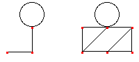
3.1.1 By Theorem 3.1.3, the number of vertices with odd degrees must be an even number. Therefore the second and third combinations are impossible. The following graphs realize the first and the fifth combinations.

In general, the condition for a list of numbers to be the degrees of some graph is that the number of odd numbers in the list is even. Specifically, let 2a₁, 2a₂, …, 2a_m, 2b₁ + 1, 2b₂ + 1, …, 2b_2n + 1 be such a list. Then we may start with m + 2n vertices V₁, V₂, …, V_m, W₁, W₂, .., W_2n. We draw a_i loops at V_i, b_i loops at W_i. Then we draw one edge between each pair W_2i, W_2i+1. The result is a graph with given list as degrees.

The condition for a list of numbers 1, 1, …, 1, 2, 2, …, 2, a₁, a₂, …, a_n (where the number of 1 is k, the number of 2 is l, and a_i > 2) to be the degrees of a connected graph is the evenness of the number of odd numbers and

a₁ + a₂ + … + a_n - 2n + 2 ≥ k.

The key for proving this is the following fact: Suppose A is a collection of natural numbers, and a, b ∈ A, a > 2, b ≥ 2. Suppose B is obtained by replacing a and b in A by a - 1 and b + 1. Then A can be realized by a connected graph if and only if B can be realized by a graph.

To prove the fact, let G be a graph whose degrees is A. Let V and W be vertices in G such that deg_G(V) = a, deg_G(W) = b. Since G is connected, we can find a path α connecting V to W. If α comes back to V before reaching W, then α is broken into two paths, the first part β starts and ends at V, and the second part γ connecting V to W. By (repeatedly, if necessary) using γ in place of α, we may assume that α actually does not come back to V. Thus we are in the situation like the left of the picture below, in which the path α is painted red, and there is only one red edge at V.

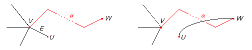
Since a > 2, there are other edges at V not belonging to α. Let one such edge be E, connecting V to U. Then by deleting E and adding an edge between U and W, we get a new graph G' on the right. Because of α, G' is still connected. Moreover, the only changes of degree in going from G to G' are: deg_G'(V) = a - 1, deg_G'(W) = b + 1. Thus G' is a connected graph with B as degrees.

Having proved the fact, we can now go back to our original question. Suppose A = {1, 1, …, 1, 2, 2, …, 2, a₁, a₂, …, a_n} is the degrees of a connected graph. By taking a = a₁ and b = a₂ in the fact, we see that B = {1, 1, …, 1, 2, 2, …, 2, a₁-1, a₂ + 1, …, a_n} is also the degrees of another connected graph. Continuing the process, we eventually modify a₁, a₂, …, a_n into 2, 2, …, 2, b, where

b = (a₁ - 2) + (a₂ - 2) + … + (a_n-1 - 2) + a_n = a₁ + a₂ + … + a_n - 2n + 2.

Eventually A becomes a set R = {1, 1, …, 1, 2, 2, …, 2, b}, where the number of 1 is k, th number of 2 is l + n -1. The degree 2 points are "removable". For the graph to be connected, the degree 1 points must all be connected to the degree b point. This implies b ≥ k.

3.2.1 The second picture contains four points of degree 3, so that the path cannot be found. A path can be found for the the other pictures.

3.2.2 All four vertices of the Königsberg graph have odd degree. If we add an edge between any of the two vertices, then the two vertices will have even orders and the remaining two still have odd orders. Therefore Euler's problem can be solved for the new graph. Practially, this means that Euler's problem can be solved if we build one bridge between any two parts of the four parts of Königsberg.

3.2.3 Suppose the number of vertices with odd degrees is N. Then by Theorem 3.1.3, N is an even number. If we connect two such points by a new edge, then the number is decreased to N - 2. Therefore if N > 2, then we may add (N - 2)/2 number of edges to get a connected graph with only two vertices of odd degrees, for which Euler's problem has solution. Therefore we conclude the following

If N = 0 or 2, then no need to add edges.
If N > 2, then we need to add (N - 2)/2 edges.

3.2.4 By a proof similar to the necessary part of Theorem 3.1.2, if we can traverse the graph G in two trips, then G has at most two connected components, the number of odd order degree vertices must be N = 0, 2 or 4, and we must be in one of the following situation

G is connected and N = 0 or 2, then one trip is enough.
G is connected and N = 4, then two trips are enough, and the the trips begin and end at odd degree vertices.
G has two connected components and N = 0 or 2, then the odd order vertices are in the same component, and two trips (one in each component) is enough.
G has two connected components and N = 4, then each component has two odd order vertices, and two trips (one in each component) is enough.

Next we prove the situations described above are sufficient for two trips. Again this can be done by inducting on the number of edges. By the sufficient part of Theorem 3.1.2, we can traverse the graph in no more than two trips in the all except the second case. So only the second case needs to be proved.

Assume G is connected and has 4 vertices of odd degree. Similar to the proof of the sufficient part of Theorem 3.1.2, let V be one of the odd degree vertex and let E be one edge with V as one end. If deleting E from G gives us a connected graph G', then by counting the degree of vertices in G', we see that G' is in either the first or the second situation described above, and the proof can be finished by induction. If deleting E from G gives us a non-connected graph, then the new graph must have two connected components G₁ and G₂, and we may assume V lies in G₁. Since the numbers of odd order vertices in G₁ and G₂ are even, by simple computations of degrees, we find there are two possibilities

G₁ has no vertices of odd order, G₂ has either 2 or 4 vertices of odd order.
G₁ has 2 vertices of odd order, G₂ has either 0 or 2 vertices of odd order. In case G₂ has 2 vertices of odd order, one such vertex is the other end of the edge E.

In the first case, we can replace E by another edge E' in G that has V as one end. Then by Lemma 3.2.1, deleting E' from G gives us a connected graph, and induction can still be used. In the second case, we can traverse G₁ and G₂ by one trip each, with end points being vertices of odd degree or the trip being a cycle. From the two trips, it is very easy to construct two trips traversing the whole G.

Math4225 Homework 2