4.2.3 Connection 1-form
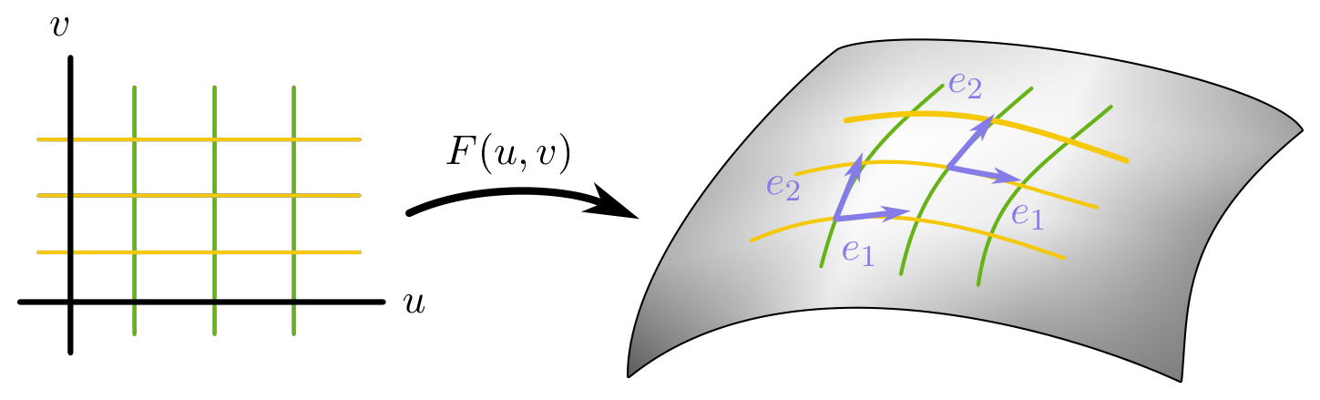
Let \(\Sigma^2\subset\mathbb{R}^3\) be a regular surface, locally parametrized by \(F(u^1,u^2)\). Locally, one can consider a pair of unit tangent vector fields \(\{e_1,e_2\}\) which are orthogonal to each other. For instance, one way to construct such a pair is by the Gram-Schmidt process: \[e_1:=\frac{\frac{\partial F}{\partial u^1}}{\left|\frac{\partial F}{\partial u^1}\right|},\qquad e_2:=\frac{\frac{\partial F}{\partial u^2}-\frac{g_{21}}{g_{11}}\frac{\partial F}{\partial u^1}}{\left|\frac{\partial F}{\partial u^2}-\frac{g_{21}}{g_{11}}\frac{\partial F}{\partial u^1}\right|}.\] Such a pair of tangent vector fields (locally defined) is called an orthonormal frame.
Fix any orthonormal frame \(\{e_1,e_2\}\). For each \(i,j\in\{1,2\}\), we define a differential 1-form \(\omega_{ij}\) so that for any vector field \(X\): \[\omega_{ij}(X):=g(e_i,\nabla_X e_j),\] where \(\nabla\) is the covariant derivative. This \(\omega_{ij}\) is called the connection 1-form.
Take the unit sphere, locally parametrized by \(F(\theta,\varphi)=(\sin\varphi\cos\theta,\sin\varphi\sin\theta,\cos\varphi)\).
Since \(\frac{\partial F}{\partial\theta}\) and \(\frac{\partial F}{\partial\varphi}\) are orthogonal, we take \(e_1:=\frac{1}{\sin\varphi}\frac{\partial F}{\partial\theta}\) and \(e_2:=\frac{\partial F}{\partial\varphi}\).
Then the connection 1-form \(\omega_{12}\) is found as follows. Using \(g_{\theta\theta}=\sin^2\varphi\), \(g_{\theta\varphi}=g_{\varphi\theta}=0\), \(g_{\varphi\varphi}=1\), and \(\Gamma^\theta_{\theta\varphi}=\frac{\cos\varphi}{\sin\varphi}\), one computes \[\omega_{12}\!\left(\frac{\partial F}{\partial\theta}\right)=\frac{1}{\sin\varphi}\Gamma^\theta_{\theta\varphi}g_{\theta\theta}=\cos\varphi,\qquad\omega_{12}\!\left(\frac{\partial F}{\partial\varphi}\right)=0.\] Therefore \(\omega_{12}=\cos\varphi\,d\theta\).
Verify that \(\omega_{12}\!\left(\frac{\partial F}{\partial\varphi}\right)=0\).
Compute \(d\omega_{12}\), and evaluate the integral \(\int_{S^2}d\omega_{12}\). Remark: we will see later that this integral is closely related to the Gauss-Bonnet's Theorem.
By the product rule \(D_X\langle e_i,e_j\rangle=\langle\nabla_X e_i,e_j\rangle+\langle e_i,\nabla_X e_j\rangle\) and the fact that \(\langle e_i,e_j\rangle=\delta_{ij}\) is constant, we easily see that \[\omega_{ij}=-\omega_{ji}.\] In particular, \(\omega_{11}=\omega_{22}=0\).
The connection 1-form \(\omega_{ij}\)'s depend on the choice of orthonormal frame \(\{e_1,e_2\}\).