2.1.1 Regular Parametrizations
In Multivariable Calculus, we expressed a surface in \(\R^3\) in two major ways, namely using a parametrization \(\bF(u,v)\) or by a level set \(f(x,y,z)=0\). In this section, let us first focus on the former.
Recall that in MATH 2023 we can use a parametrization \(\bF(u,v)\) to describe a surface in \(\R^3\) and to calculate various geometric and physical quantities such as surface areas, surface integrals and surface flux. To start the course, we first look into several technical and analytical aspects concerning \(\bF(u,v)\), such as their domains and images, their differentiability, etc. In the past, we could usually cover (or almost cover) a surface by a single parametrization \(\bF(u,v)\). Take the unit sphere as an example. We learned that it can be parametrized with the help of spherical coordinates:
\[\bF(\theta,\varphi)=(\sin\varphi\cos\theta,\ \sin\varphi\sin\theta,\ \cos\varphi)\]
where \(0<\theta<2\pi\) and \(0<\varphi<\pi\). This parametrization covers almost every part of the sphere (except the north and south poles, and a half great circle connecting them). In order to cover the whole sphere, we need more parametrizations, such as \(\bG(\theta,\varphi)=(\sin\varphi\cos\theta,\sin\varphi\sin\theta,\cos\varphi)\) with domain \(-\pi<\theta<\pi\) and \(0<\varphi<\pi\). Since the image of either \(\bF\) or \(\bG\) does not cover the whole sphere (although almost), from now on we call them local parametrizations.
Consider a subset \(M\subset\R^3\). A function \(\bF(u,v):U\to O\) from an open subset \(U\subset\R^2\) onto an open subset \(O\subset M\) is called a \(C^k\) local parametrization (or a \(C^k\) local coordinate chart) of \(M\) (where \(k\ge 1\)) if all of the following holds:
- \(\bF:U\to\R^3\) is \(C^k\) when the codomain is regarded as \(\R^3\).
- \(\bF:U\to O\) is a homeomorphism, meaning that \(\bF:U\to O\) is bijective, and both \(\bF:U\to O\) and \(\bF^{-1}:O\to U\) are continuous.
- For all \((u,v)\in U\), the cross product \(\displaystyle \pdF{u}\times\pdF{v}\neq \mathbf{0}.\)
The coordinates \((u,v)\) are called the local coordinates of \(M\). If \(\bF:U\to M\) is of class \(C^k\) for any integer \(k\), then \(\bF\) is said to be a \(C^\infty\) (or smooth) local parametrization.
A subset \(M\subset\R^3\) is called a \(C^k\) surface, where \(k\in\N\cup\{\infty\}\), in \(\R^3\) if at every point \(p\in M\), there exists an open subset \(U\subset\R^2\), an open subset \(O\subset M\) containing \(p\), and a \(C^k\) local parametrization \(\bF:U\to O\) which satisfies all three conditions stated in Definition 2.1.
We say \(M\) is a regular surface in \(\R^3\) if it is a \(C^\infty\) surface.
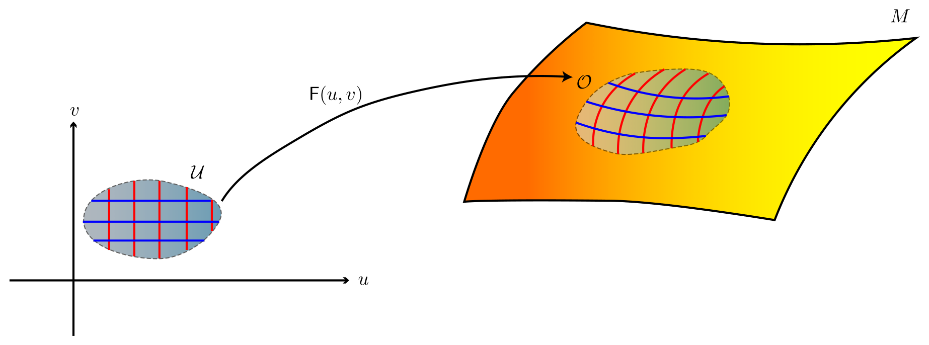
To many students, the definition of regular surfaces looks daunting at first glance – especially condition (3). One way to make better sense of it is to look at some examples and understand why each of the three conditions is needed in the definition.
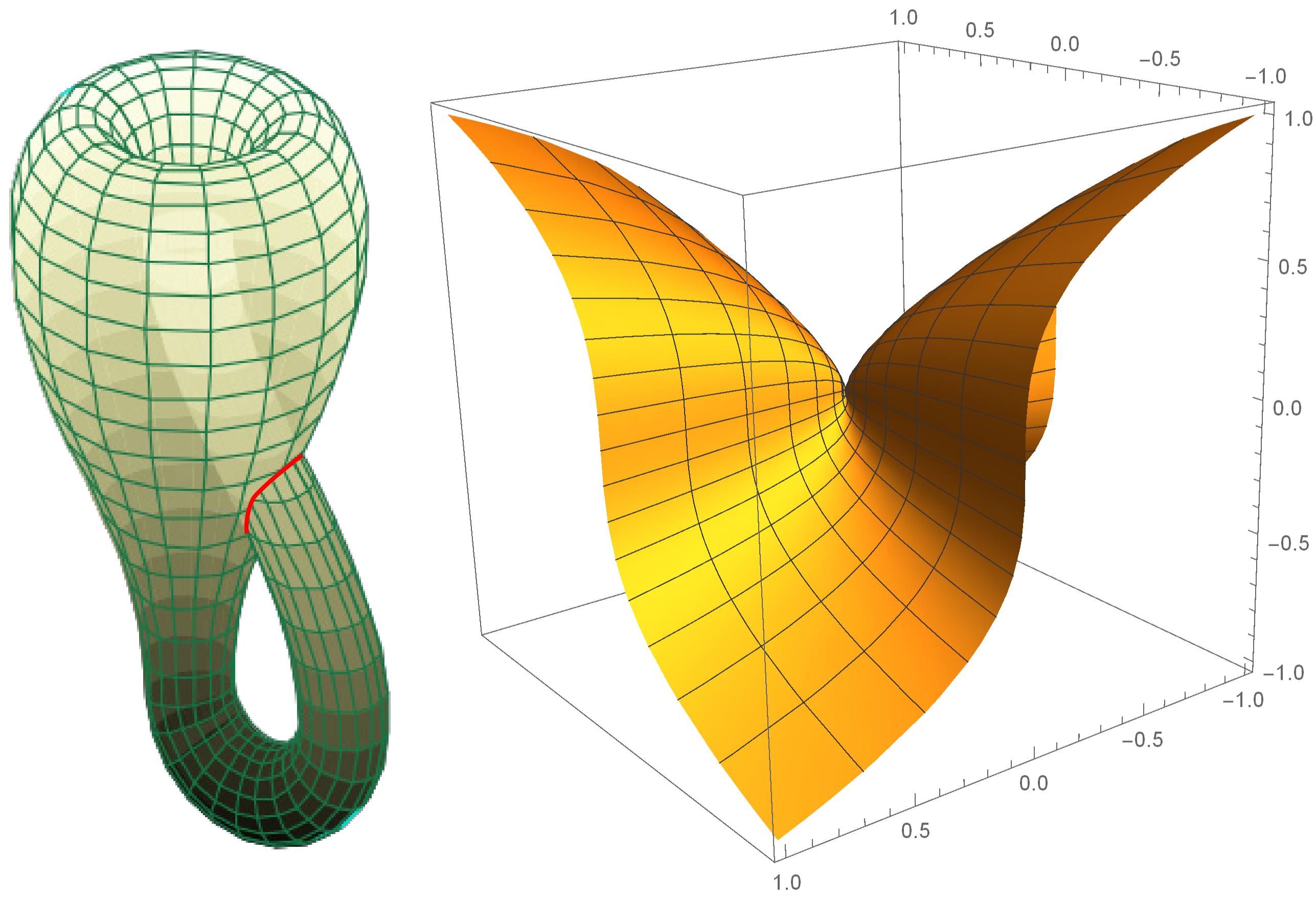
The motivation behind condition (1) in the definition is that we are studying differential topology/geometry and so we want the parametrization to be differentiable as many times as we like. Condition (2) rules out surfaces that have self-intersection such as the Klein bottle (see Figure 2.2a). Finally, condition (3) guarantees the existence of a unique tangent plane at every point on \(M\) (see Figure 2.2b for a non-example).
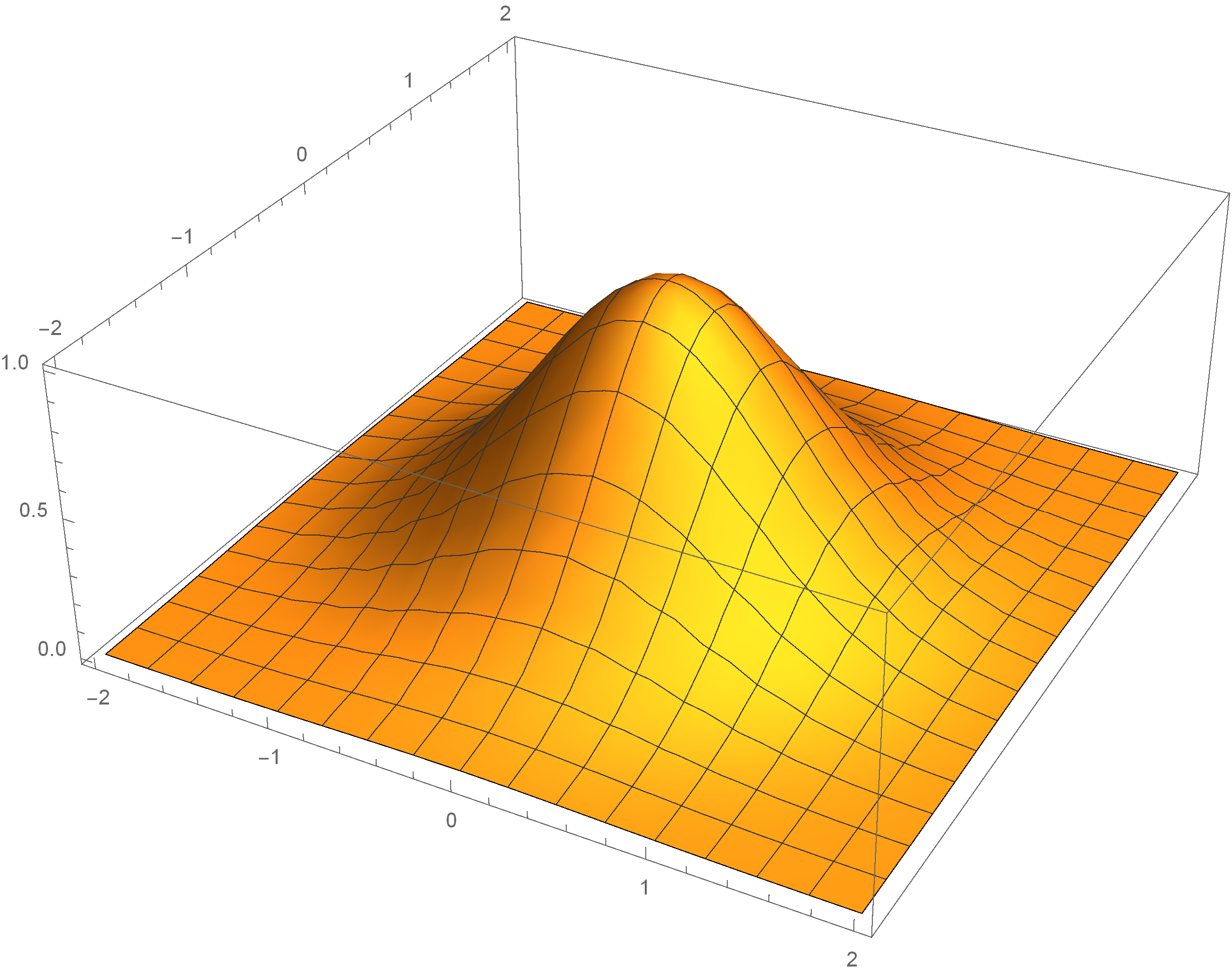
Consider a smooth function \(f(u,v):U\to\R\) defined on an open subset \(U\subset\R^2\). The graph of \(f\), denoted by \(\Gamma_f\), is the subset \(\{(u,v,f(u,v)):(u,v)\in U\}\) of \(\R^3\). One can parametrize \(\Gamma_f\) by a global parametrization \(\bF(u,v)=(u,v,f(u,v))\).
Condition (1) holds because \(f\) is given to be smooth. For condition (2), \(\bF\) is clearly one-to-one, and the image of \(\bF\) is the whole graph \(\Gamma_f\). Regarding it as a map \(\bF:U\to\Gamma_f\), the inverse map \(\bF^{-1}(x,y,z)=(x,y)\) is clearly continuous. Therefore, \(\bF:U\to\Gamma_f\) is a homeomorphism. To verify condition (3), we compute the cross product:
\[\pdF{u}\times\pdF{v}=\left(-\pd{f}{u},\,-\pd{f}{v},\,1\right)\neq\mathbf{0}\]
for all \((u,v)\in U\). Therefore, \(\bF\) is a smooth local parametrization of \(\Gamma_f\). Since the image of this single smooth local parametrization covers all of \(\Gamma_f\), we conclude that \(\Gamma_f\) is a regular surface. \(\square\)
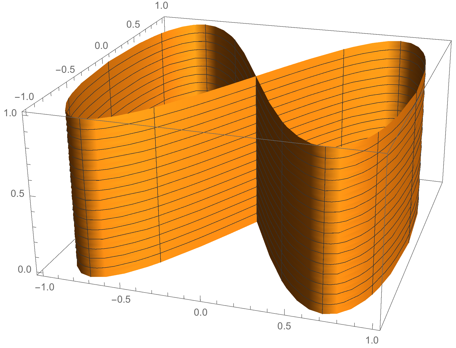
Show that \(\bF(u,v):(0,2\pi)\times(0,1)\to\R^3\) defined by \(\bF(u,v)=(\sin u,\sin 2u,v)\) satisfies conditions (1) and (3) in Definition 2.1, but not condition (2). [Hint: Try to show \(\bF^{-1}\) is not continuous by finding a diverging sequence \(\{(u_n,v_n)\}\) such that \(\{\bF(u_n,v_n)\}\) converges. See Figure 2.4 for reference.]
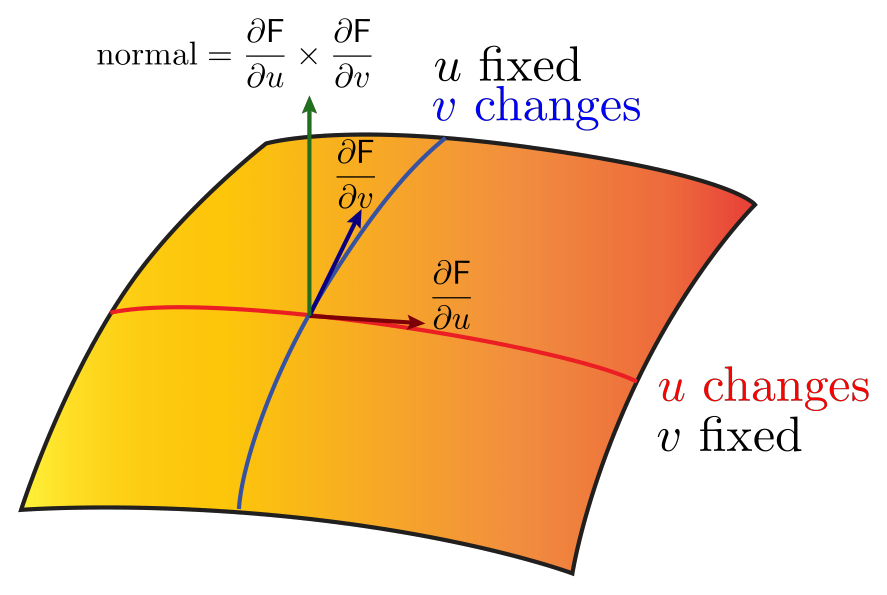
In Figure 2.3, one can observe that there are two families of curves on the surface. These curves, often called coordinate curves, are obtained by varying one of the \((u,v)\)-variables while keeping the other constant. Precisely, they are the curves represented by \(\bF(u,v_0)\) and \(\bF(u_0,v)\) where \(u_0\) and \(v_0\) are fixed. As such, the partial derivatives \(\pdF{u}(p)\) and \(\pdF{v}(p)\) give a pair of tangent vectors on the surface at point \(p\). Therefore, their cross product \(\pdF{u}(p)\times\pdF{v}(p)\) is a normal vector to the surface at point \(p\) (see Figure 2.5). Here we have abused the notations for simplicity: \(\pdF{u}(p)\) means \(\pdF{u}\) evaluated at \((u,v)=\bF^{-1}(p)\). Similarly for \(\pdF{v}(p)\).
Condition (3) requires that \(\pdF{u}\times\pdF{v}\) is everywhere non-zero in the domain of \(\bF\). An equivalent statement is that the vectors \(\big\{\pdF{u}(p),\pdF{v}(p)\big\}\) are linearly independent for any \(p\in\bF(U)\).
In \(\R^3\), the unit sphere \(S^2\) centered at the origin can be represented by the equation \(x^2+y^2+z^2=1\), or in other words, \(z=\pm\sqrt{1-x^2-y^2}\). We can parametrize the upper and lower hemisphere by two separate local maps:
\[\bF_1(u,v)=(u,v,\sqrt{1-u^2-v^2}):B_1(0)\subset\R^2\to S^2_+\]\[\bF_2(u,v)=(u,v,-\sqrt{1-u^2-v^2}):B_1(0)\subset\R^2\to S^2_-\]
where \(B_1(0)=\{(u,v):u^2+v^2<1\}\) is the open unit disk in \(\R^2\) centered at the origin, and \(S^2_+\) and \(S^2_-\) are the upper and lower hemispheres of \(S^2\) respectively. Since \(B_1(0)\) is open, the functions \(\pm\sqrt{1-u^2-v^2}\) are smooth, and according to the previous example both \(\bF_1\) and \(\bF_2\) are smooth local parametrizations.
However, not all points on the sphere are covered by \(S^2_+\) and \(S^2_-\), since points on the equator are not. In order to show that \(S^2\) is a regular surface, we need to write down more smooth local parametrization(s) so that each point on the sphere can be covered by at least one smooth local parametrization chart. One can construct four more smooth local parametrizations (left, right, front and back) similar to \(\bF_1\) and \(\bF_2\) (see Figure 2.6). It is left as an exercise for readers to write down the other four parametrizations. These six parametrizations are all smooth and they cover the whole sphere. Therefore, it shows the sphere is a regular surface. \(\square\)
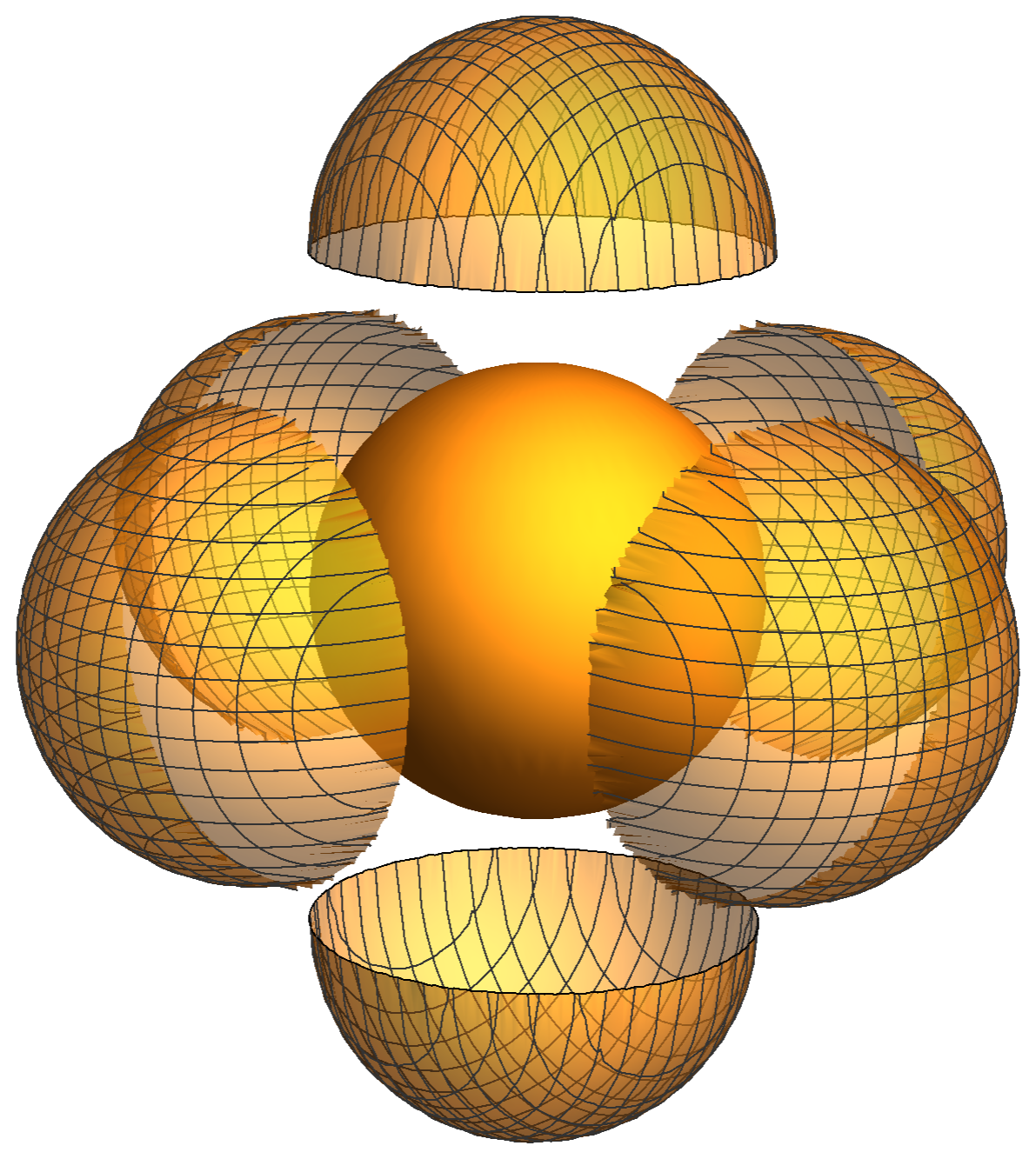
Write down the left, right, front and back parametrizations \(\bF_i\) (\(i=3,4,5,6\)) of the sphere as shown in Figure 2.6. Indicate clearly the domain and range of each \(\bF_i\).
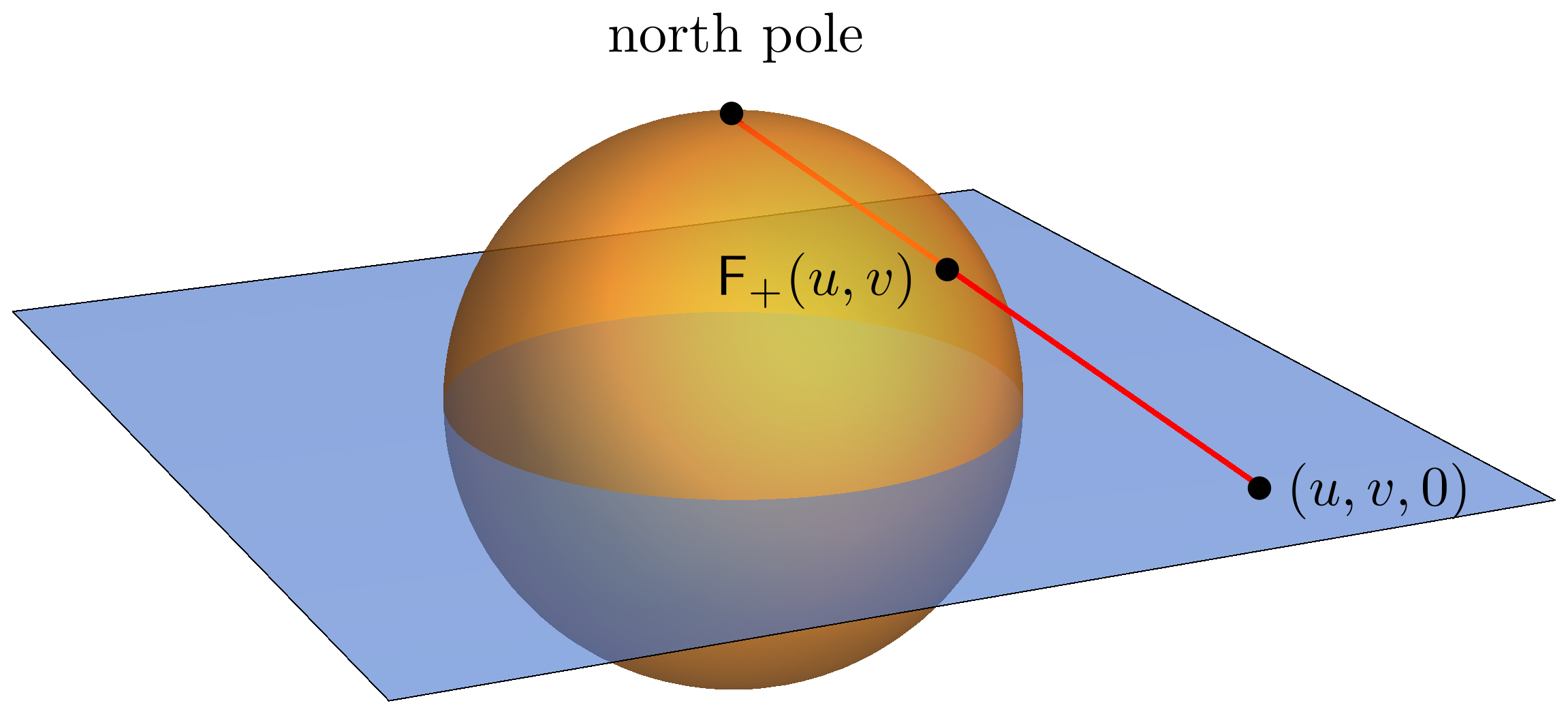
We can in fact cover the sphere by just two smooth local parametrizations described below. Define \(\bF_+(u,v):\R^2\to S^2\setminus\{(0,0,1)\}\) where:
\[\bF_+(u,v)=\left(\frac{2u}{u^2+v^2+1},\ \frac{2v}{u^2+v^2+1},\ \frac{u^2+v^2-1}{u^2+v^2+1}\right)\]
It is called the stereographic parametrization of the sphere (see Figure 2.7), which assigns each point \((u,v,0)\) on the \(xy\)-plane of \(\R^3\) to a point where the line segment joining \((u,v,0)\) and the north pole \((0,0,1)\) intersects the sphere. Clearly \(\bF_+\) is a smooth function. We leave it as exercise for readers to verify that \(\bF_+\) satisfies condition (3) and that \(\bF_+^{-1}:S^2\setminus\{(0,0,1)\}\to\R^2\) is given by:
\[\bF_+^{-1}(x,y,z)=\left(\frac{x}{1-z},\ \frac{y}{1-z}\right).\]
As \(z\neq 1\) for every \((x,y,z)\) in the domain of \(\bF_+^{-1}\), it is a continuous function. Therefore, \(\bF_+\) is a smooth local parametrization. The inverse map \(\bF_+^{-1}\) is commonly called the stereographic projection of the sphere.
Note that the range of \(\bF_+\) does not include the point \((0,0,1)\). In order to show that the sphere is a regular surface, we need to cover it by another parametrization \(\bF_-:\R^2\to S^2\setminus\{(0,0,-1)\}\) which assigns each point \((u,v,0)\) on the \(xy\)-plane to a point where the line segment joining \((u,v,0)\) and the south pole \((0,0,-1)\) intersects the sphere. It is an exercise for readers to write down the explicit parametrization \(\bF_-\). \(\square\)
Verify that \(\bF_+\) in Example 2.5 satisfies condition (3) in Definition 2.1, and that the inverse map \(\bF_+^{-1}:S^2\setminus\{(0,0,1)\}\to\R^2\) is given as stated. [Hint: Write down \(\bF_+(u,v)=(x,y,z)\) and solve \((u,v)\) in terms of \((x,y,z)\). Begin by finding \(u^2+v^2\) in terms of \(z\).] Furthermore, write down explicitly the map \(\bF_-\) described in Example 2.5, and find its inverse map \(\bF_-^{-1}\).
Find smooth local parametrizations which together cover the whole ellipsoid \(\dfrac{x^2}{a^2}+\dfrac{y^2}{b^2}+\dfrac{z^2}{c^2}=1\) where \(a,b\) and \(c\) are positive constants.
Let \(M\) be the cylinder \(\{(x,y,z)\in\R^3:x^2+y^2=1\}\). The purpose of this exercise is to construct a smooth local parametrization analogous to the stereographic parametrization in Example 2.5: Consider the unit circle \(x^2+y^2=1\) on the \(xy\)-plane. For each point \((u,0)\) on the \(x\)-axis, we construct a straight-line joining the point \((0,1)\) and \((u,0)\). This line intersects the unit circle at a unique point \(p\). Denote the \(xy\)-coordinates of \(p\) by \((x(u),y(u))\).
- Find the coordinates \((x(u),y(u))\) in terms of \(u\).
- Define \(\bF_1(u,v)=(x(u),y(u),v)\) with \(\R^2\) as its domain. Describe the image of \(\bF_1\).
- Denote \(O_1\) to be the image of \(\bF_1\). Verify that \(\bF_1:\R^2\to O_1\) is a smooth local parametrization of \(M\).
- Construct another smooth local parametrization \(\bF_2\) such that the images of \(\bF_1\) and \(\bF_2\) cover the whole surface \(M\) (hence establish that \(M\) is a regular surface).
Let’s also look at a non-example of smooth local parametrizations. Consider the map \(\bG(u,v)=(u^3,v^3,0)\), \((u,v)\in\R\times\R\). It is a smooth, injective map from \(\R^2\) onto the \(xy\)-plane \(\Pi\) of \(\R^3\), i.e. \(\bG:\R^2\to\Pi\). However, it can be computed that \(\pd{\bG}{u}(0,0)=\pd{\bG}{v}(0,0)=\mathbf{0}\) and so condition (3) in Definition 2.1 does not hold. The map \(\bG\) is not a smooth local parametrization of \(\Pi\). However, note that \(\Pi\) is a regular surface because \(\bF(u,v)=(u,v,0)\) is a smooth global parametrization of \(\Pi\), even though \(\bG\) is not a “good” parametrization.
In order to show \(M\) is a regular surface, what we need is to show at every point \(p\in M\) there is at least one smooth local parametrization \(\bF\) near \(p\). However, to show that \(M\) is not a regular surface, one then needs to come up with a point \(p\in M\) such that there is no smooth local parametrization near that point \(p\) (which may not be easy).