Overview
In this section we introduce another important 2-tensor on \(\Tp{p}\Sigma\), the second fundamental form \(h\). While the first fundamental form \(g\) encodes information about angle, length and area, the second fundamental form encodes information about various curvatures.
We will see in subsequent sections that curvatures of a regular hypersurface are, roughly speaking, determined by rates of change of tangent and normal vectors just like the case for regular curves. Let’s first talk about the normal vector – or in differential geometry jargon – the Gauss Map.
Given a regular hypersurface \(\Sigma\) in \(\mathbb{R}^{n+1}\) with \(F(u_i): \mathcal{U}\subset\mathbb{R}^n\to\Sigma\) as one of its local parametrizations. Let \(p\in M\), the orthogonal complement of the tangent space \(\Tp{p}\Sigma\) in \(\mathbb{R}^{n+1}\) is a 1-dimensional vector space denoted by \(N_p\Sigma\). There are exactly two unit vectors in \(N_p\Sigma\). In dimension 2 (i.e. regular surfaces), \(\pdF{u}(p)\) and \(\pdF{v}(p)\) are two linearly independent tangents at \(p\), and so the two unit normals are given by \[ \nu(p) = \frac{\pdF{u}(p)\times\pdF{v}(p)}{|\pdF{u}(p)\times\pdF{v}(p)|} \quad \text{or} \quad -\frac{\pdF{u}(p)\times\pdF{v}(p)}{|\pdF{u}(p)\times\pdF{v}(p)|}. \] See the result from Exercise 7.6 for higher dimensional hypersurfaces.
Consider the unit sphere \(S^2(1)\) with smooth local parametrization: \[ F(u,v) = (\sin u\cos v,\, \sin u\sin v,\, \cos u), \quad (u,v)\in(0,\pi)\times(0,2\pi). \] It is straight-forward to compute that: \[ \pd{\mathbf{F}}{u}\times\pd{\mathbf{F}}{v} = (\sin^2 u\cos v,\, \sin^2 u\sin v,\, \sin u\cos u), \] \[ \left|\pd{\mathbf{F}}{u}\times\pd{\mathbf{F}}{v}\right| = \sin u, \] \[ \nu(u,v) = (\sin u\cos v,\, \sin u\sin v,\, \cos u) = F(u,v). \] This unit normal vector \(\nu\) is outward-pointing.
Suppose \(\Sigma^2\subset\mathbb{R}^3\) is a regular surface in \(\mathbb{R}^3\), with two local parametrizations \(F(u_1,u_2)\) and \(G(v_1,v_2)\), then we have the normal vector is independent of the choice of local parametrizations up to a sign, i.e. \[ \frac{\pd{\mathbf{F}}{u_1}(p)\times\pd{\mathbf{F}}{u_2}(p)}{\left|\pd{\mathbf{F}}{u_1}(p)\times\pd{\mathbf{F}}{u_2}(p)\right|} = \pm\,\frac{\pd{G}{v_1}(p)\times\pd{G}{v_2}(p)}{\left|\pd{G}{v_1}(p)\times\pd{G}{v_2}(p)\right|}. \]
Given a regular hypersurface, there are always two choices of normal vector at each point. For a sphere, once the normal vector direction is chosen, it is always consistent with your choice when we move the normal vector across the sphere. We call it an orientable hypersurface if there exists a continuous choice of unit normal vector across the whole hypersurface. See Chapter 7 for more thorough discussions on orientability.
When \(\Sigma\) is an orientable regular hypersurface, the chosen unit normal vector \(\nu\) can then be regarded as a map \(\nu: \Sigma \to S^n\). We call this map as:
Suppose \(\Sigma\) is an orientable regular hypersurface. The Gauss map of \(\Sigma\) is a smooth function \(\nu: \Sigma \to S^n\) such that for any \(p\in\Sigma\), the output \(\nu(p)\) is a unit normal vector of \(\Sigma\) at \(p\). Here \(S^n\) is the unit \(n\)-sphere in \(\mathbb{R}^{n+1}\).
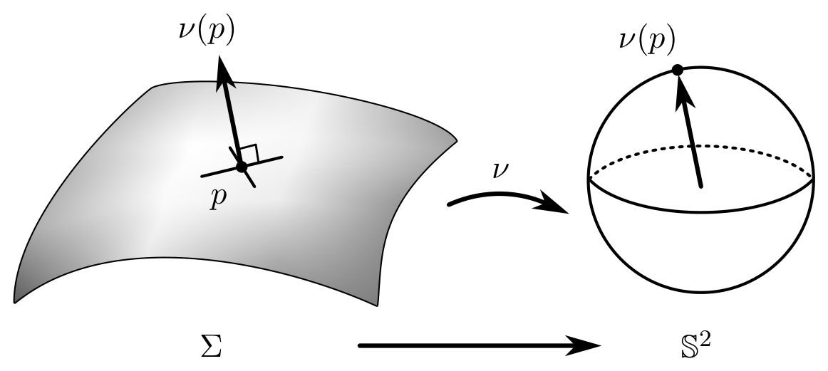
As computed in Example 3.7, the Gauss map \(\nu\) for the unit sphere \(S^2\) is given by \(F\) (assuming the outward-pointing convention is observed). The Gauss map \(\nu\) for a sphere with radius \(R\) centered at the origin in \(\mathbb{R}^3\) is given by \(\frac{1}{R}F\). For a plane \(\Pi\), the unit normal vector at each point is the same, so \(\nu(p)\) is a constant vector independent of \(p\). A unit cylinder with \(z\)-axis as its central axis has Gauss map \(\nu(u,v) = (\cos u, \sin u, 0)\); its image in \(S^2\) is the equator.
It is not difficult to see that the image of the Gauss map \(\nu\), which is a subset of \(S^2\), is related to how “spherical” or “planar” the surface looks. The smaller the image, the more planar it is.
The curvature of a regular curve is a scalar function \(\kappa(p)\). Since a curve is one dimensional, we can simply use one single value to measure the curvature at each point. However, a regular hypersurface has arbitrary dimensions and hence has higher degree of freedom than curves. It may bend by a different extent along different directions. As such, there are various notions of curvatures for regular hypersurfaces. We first talk about the normal curvature, which is fundamental to many other notions of curvatures.
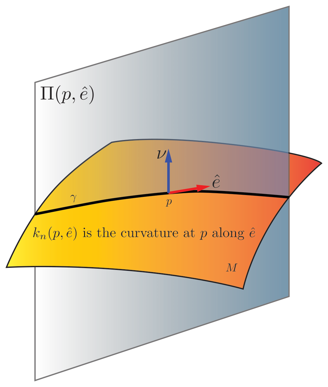
Let \(\Sigma\) be an orientable regular hypersurface with its Gauss map denoted by \(\nu\). At each point \(p\in\Sigma\), we pick a unit tangent vector \(\hat{e}\) in \(\Tp{p}\Sigma\). Heuristically, the normal curvature at \(p\) measures the curvature of the surface along a direction \(\hat{e}\). Precisely, we define:
Let \(\Sigma\) be an orientable regular hypersurface with Gauss map \(\nu\). For each point \(p\in\Sigma\), and any unit tangent vector \(\hat{e}\in\Tp{p}\Sigma\), we let \(\Pi_p(\nu,\hat{e})\) be the plane in \(\mathbb{R}^{n+1}\) passing through \(p\) and parallel to both \(\nu(p)\) and \(\hat{e}\) (see Figure 3.2). Let \(\gamma\) be the curve of intersection of \(\Sigma\) and \(\Pi_p(\nu,\hat{e})\). The normal curvature at \(p\) in the direction of \(\hat{e}\) of \(\Sigma\), denoted by \(k_n(p,\hat{e})\), is defined to be the signed curvature \(k(p)\) of the curve \(\gamma\) at \(p\) with respect to the Gauss map \(\nu\).
Since \(k_n(p,\hat{e})\) is defined using the Gauss map \(\nu\), which always comes with two possible choices for any orientable regular surface, the normal curvature depends on the choice of the Gauss map \(\nu\). If the opposite unit normal is chosen to be the Gauss map, the normal curvature will differ by a sign.
We will first make sense of normal curvatures through elementary examples, then we will prove a general formula for computing normal curvatures.
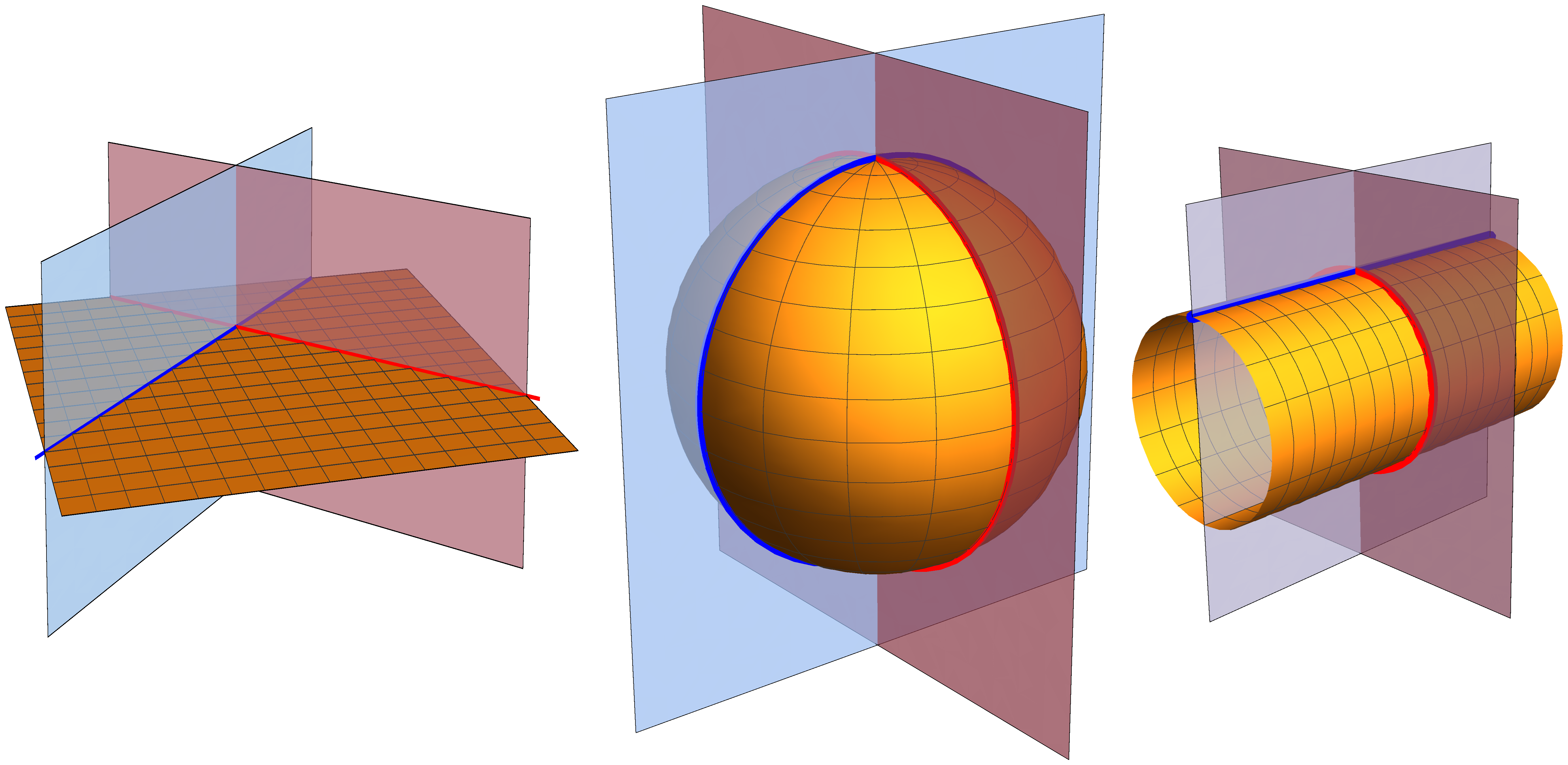
Let \(P\) be any plane in \(\mathbb{R}^3\). For any point \(p\in P\) and unit tangent \(\hat{e}\in\Tp{p}P\), the plane \(\Pi_p(\nu,\hat{e})\) must cut through \(P\) along a straight-line \(\gamma\). Since \(\gamma\) has curvature \(0\), we have: \[ k_n(p,\hat{e}) = 0 \] for any \(p\in P\) and \(\hat{e}\in\Tp{p}P\). See Figure 3.3a.
Let \(S^2(R)\) be the sphere with radius \(R\) centered at the origin in \(\mathbb{R}^3\) with Gauss map \(\nu\) taken to be inward-pointing. For any point \(p\in S^2\) and \(\hat{e}\in\Tp{p}S^2(R)\), the plane \(\Pi_p(\nu,\hat{e})\) cuts \(S^2(R)\) along a great circle (with radius \(R\)). Since a circle with radius \(R\) has constant curvature \(\frac{1}{R}\), we have: \[ k_n(p,\hat{e}) = \frac{1}{R} \] for any \(p\in S^2(R)\) and \(\hat{e}\in\Tp{p}S^2(R)\). See Figure 3.3b.
Let \(M\) be the (infinite) cylinder of radius \(R\) with \(x\)-axis as the central axis with outward-pointing Gauss map \(\nu\). Given any \(p\in M\), if \(\hat{e}_x\) is the unit tangent vector at \(p\) parallel to the \(x\)-axis, then \(\Pi_p(\nu,\hat{e}_x)\) cuts the cylinder \(M\) along a straight-line. Therefore: \[ k_n(p,\hat{e}_x) = 0 \] for any \(p\in M\). See the blue curve in Figure 3.3c.
On the other hand, if \(\hat{e}_{yz}\) is a horizontal unit tangent vector at \(p\), then \(\Pi_p(\nu,\hat{e}_{yz})\) cuts \(M\) along a circle with radius \(R\). Therefore: \[ k_n(p,\hat{e}_{yz}) = -\frac{1}{R} \] for any \(p\in M\). See the red curve in Figure 3.3c. Note that the tangent vector of the curve is moving away from the outward-pointing \(\nu\), which explains the negative sign. For any other choice of unit tangent \(\hat{e}\) at \(p\), the normal curvature along \(\hat{e}\) may vary between \(0\) and \(-\frac{1}{R}\).
In the above examples, the normal curvatures \(k_n(p,\hat{e})\) are easy to find since the curve of intersection between \(\Pi_p(\nu,\hat{e})\) and the surface is either a straight line or a circle. Generally speaking, the curve of intersection may be of arbitrary shape such as an ellipse, and sometimes it is not even easy to identify what curve it is. Fortunately, it is possible to compute \(k_n(p,\hat{e})\) for any given unit tangent \(\hat{e}\) in a systematic way. Next we derive an expression of \(k_n(p,\hat{e})\), which will motivate the definition of the second fundamental form and Weingarten’s map (also known as the shape operator).
Let \(\Sigma\) be the regular hypersurface in \(\mathbb{R}^{n+1}\) with Gauss map \(\nu\). Fix \(p\in\Sigma\) and a unit vector \(\hat{e}\in\Tp{p}\Sigma\) which is locally expressed as \(\hat{e} = X^i \pdF{u_i}\), then the normal curvature of \(\Sigma\) at \(p\) along \(\hat{e}\) is given by: \[ k_n(p,\hat{e}) = -\left\langle\pdF{u_i},\pd{\nu}{u_j}\right\rangle X^i X^j = \left\langle\pd{^2\mathbf{F}}{u_i\partial u_j},\nu\right\rangle X^i X^j. \]
Let \(\gamma\) be the intersection curve between the plane \(\Pi_p(\nu,\hat{e})\) and \(\Sigma\). Parametrize \(\gamma\) by arc-length \(s\in(-\varepsilon,\varepsilon)\) such that \(\gamma(0)=p\) and \(|\gamma'(s)|\equiv 1\). Then \(\gamma'(0)=\hat{e} = X^i\pdF{u_i}\). Let \(\gamma^i(s)\) be functions such that \(F(\gamma^1(s),\ldots,\gamma^n(s))=\gamma(s)\). By the chain rule, \(\gamma'(s)=\pdF{u_i}\frac{d\gamma^i}{ds}\), so comparing coefficients at \(s=0\) gives \(X^i = \frac{d\gamma^i}{ds}\big|_{s=0}\).
Since \(\gamma'(s)\) is a unit tangent to \(\Sigma\), it is orthogonal to \(\nu(\gamma(s))\). Therefore: \[ k_n(p,\hat{e}) = \langle\gamma''(s),\nu(\gamma(s))\rangle\big|_{s=0} = \frac{d}{ds}\big|_{s=0}\langle\gamma'(s),\nu(\gamma(s))\rangle - \left\langle\gamma'(s),\frac{d}{ds}\nu(\gamma(s))\right\rangle\bigg|_{s=0} = 0 - \left\langle\hat{e},\,\pd{\nu}{u_i}\frac{d\gamma^i}{ds}\bigg|_{s=0}\right\rangle. \]
Substituting \(\hat{e} = X^j\pdF{u_j}\) and \(\frac{d\gamma^i}{ds}\big|_{s=0} = X^i\), we get: \[ k_n(p,\hat{e}) = -\left\langle X^j\pdF{u_j},\,X^i\pd{\nu}{u_i}\right\rangle = -X^i X^j\left\langle\pdF{u_j},\pd{\nu}{u_i}\right\rangle. \]
Finally, since \(\langle\pdF{u_j},\nu\rangle=0\), differentiating with respect to \(u_i\) gives: \[ 0 = \frac{\partial}{\partial u_i}\left\langle\pdF{u_j},\nu\right\rangle = \left\langle\pd{^2\mathbf{F}}{u_i\partial u_j},\nu\right\rangle + \left\langle\pdF{u_j},\pd{\nu}{u_i}\right\rangle, \] which implies \(k_n(p,\hat{e}) = X^i X^j\left\langle\pd{^2\mathbf{F}}{u_i\partial u_j},\nu\right\rangle\), as desired. \(\square\)
Proposition 3.14 shows that \(k_n(p,\hat{e})\) can be written as a quadratic form on \(X^i\)’s with coefficients given by \(\left\langle\pd{^2\mathbf{F}}{u_i\partial u_j},\nu\right\rangle\). This motivates the second fundamental form:
Given a regular hypersurface in \(\mathbb{R}^{n+1}\) with Gauss map \(\nu\). We define the second fundamental form of \(\Sigma\) at \(p\) to be the 2-tensor using local parametrization \(F(u_1,\ldots,u_n)\), \[ h = h_{ij}\, du^i \otimes du^j, \] where \[ h_{ij} := -\left\langle\pdF{u_i},\pd{\nu}{u_j}\right\rangle = \left\langle\pd{^2\mathbf{F}}{u_i\partial u_j},\nu\right\rangle. \]
As such, the normal curvature of \(\Sigma\) at \(p\) along \(\hat{e}\) is given by \[ k_n(p,\hat{e}) = h(\hat{e},\hat{e}). \]
Let \(\Sigma_f\) be the graph of a smooth function \(f(u_1,u_2): \mathcal{U}\to\mathbb{R}\) defined on an open subset \(\mathcal{U}\) of \(\mathbb{R}^2\), then \(\Sigma_f\) has a globally defined smooth parametrization \(F(u_1,u_2)=(u_1,u_2,f(u_1,u_2))\). By straight-forward computations: \[ \pdF{u_1} = \left(1,0,\pd{f}{u_1}\right), \quad \pdF{u_2} = \left(0,1,\pd{f}{u_2}\right), \] \[ \pd{^2\mathbf{F}}{u_i\partial u_j} = \left(0,0,\pd{^2 f}{u_i\partial u_j}\right). \] Taking the Gauss map \(\nu = \dfrac{\pdF{u_1}\times\pdF{u_2}}{|\pdF{u_1}\times\pdF{u_2}|} = \dfrac{\left(-\pd{f}{u_1},-\pd{f}{u_2},1\right)}{\sqrt{1+|\nabla f|^2}}\), the second fundamental form is given by: \[ h_{ij} = \left\langle\pd{^2\mathbf{F}}{u_i\partial u_j},\nu\right\rangle = \frac{\pd{^2 f}{u_i\partial u_j}}{\sqrt{1+|\nabla f|^2}}. \] The matrix whose \((i,j)\)-th entry is \(\pd{^2 f}{u_i\partial u_j}\) is commonly called the Hessian of \(f\), denoted \(\nabla^2 f\) or \(\nabla\nabla f\). Using this notation: \[ [h] = \frac{\nabla\nabla f}{\sqrt{1+|\nabla f|^2}}, \qquad h = \frac{1}{\sqrt{1+|\nabla f|^2}}\pd{^2 f}{u_i\partial u_j}\, du^i\otimes du^j. \]
Generalize Example 3.17 to higher dimensional graphs in \(\mathbb{R}^{n+1}\): \(x_{n+1} = f(x_1,\ldots,x_n)\). Hint: the only thing that needs to be changed is the cross product when computing \(\nu\).
Given that \(k_n(p,\hat{e})\) depends on the unit direction \(\hat{e}\in\Tp{p}\Sigma\), it is natural to ask when \(k_n(p,\hat{e})\) achieves the maximum and minimum among all unit vectors \(\hat{e}\) in \(\Tp{p}\Sigma\). It is a simple optimization problem of critical points of \(h(\hat{e},\hat{e})\) subject to \(g(\hat{e},\hat{e})=1\). We call the critical values of \(h(\hat{e},\hat{e})\) subject to \(g(\hat{e},\hat{e})=1\) to be principal curvatures and we have the following important result:
Given a regular hypersurface \(\Sigma\) in \(\mathbb{R}^{n+1}\) and fix a point \(p\in\Sigma\), the principal curvatures are eigenvalues of the linear map: \[ S_p: \Tp{p}\Sigma \to \Tp{p}\Sigma, \qquad \pdF{u_i} \mapsto (g^{jk}h_{ki})\pdF{u_j}. \] The map \(S_p\) is called the Weingarten’s map, or the shape operator.
Denote \(\hat{e} = X^i\pdF{u_i}\), then \(k_n(p,\hat{e}) = h(\hat{e},\hat{e}) = h_{ij}X^i X^j\) and \(|\hat{e}|^2 = g_{ij}X^i X^j\). To determine the principal curvatures, we use Lagrange’s multiplier to find the critical values of \(h_{ij}X^i X^j\) under the constraint \(g_{ij}X^i X^j = 1\). Here \((X^1,\ldots,X^n)\) are the variables, while \(g_{ij}\) and \(h_{ij}\) are constants.
We need to solve the system \[ \frac{\partial}{\partial X^k}(h_{ij}X^i X^j) = \lambda\frac{\partial}{\partial X^k}(g_{ij}X^i X^j), \quad k=1,\ldots,n, \quad g_{ij}X^i X^j = 1. \] Using \(\frac{\partial X^i}{\partial X^k} = \delta_{ik}\), one obtains \(h_{kj}X^j = \lambda g_{kj}X^j\) for any \(k\). \(\quad\) (3.3)
Multiplying \(g^{ik}\) (the \((i,k)\)-entry of \(g^{-1}\)) on both sides of (3.3) and summing over \(k\): \[ g^{ik}h_{kj}X^j = \lambda X^i, \] for any \(i\), i.e. \([g]^{-1}[h](X^1,\ldots,X^n)^T = \lambda(X^1,\ldots,X^n)^T\). So \(\lambda\) is an eigenvalue of \([g]^{-1}[h]\).
From (3.3), \(h_{kj}X^j X^k = \lambda g_{kj}X^j X^k = \lambda\). Therefore, if \(k_n(p,\hat{e})\) achieves its maximum or minimum, then \(k_n(p,\hat{e})=\lambda\) is an eigenvalue of \([g]^{-1}[h]\), which is the matrix representation of \(S_p\). \(\square\)
From now on we denote \(h^j_i := g^{jk}h_{ki}\) so that \(S\!\left(\pdF{u_i}\right) = h^j_i\pdF{u_j}\).
Denote the eigenvalues of \(S_p\), i.e. the principal curvatures, by \(\lambda_1(p),\ldots,\lambda_n(p)\). The maximum and minimum possible normal curvatures at \(p\) among all unit directions are two of the principal curvatures. We further define:
\[ H(p) := \lambda_1(p)+\cdots+\lambda_n(p) = \operatorname{tr}[g]^{-1}[h] \qquad (\text{mean curvature}) \] \[ K(p) := \lambda_1(p)\cdots\lambda_n(p) = \det[g]^{-1}[h] = \frac{\det[h]}{\det[g]} \qquad (\text{Gauss curvature}) \]
Consider the surfaces in Figure 3.3.
For the plane, \(k_n(p,\hat{e})=0\) at any point \(p\) along any tangent direction \(\hat{e}\). Therefore, the two principal curvatures are \(0\), and hence both Gauss and mean curvatures are zero too.
For the round sphere with radius \(R\), \(k_n(p,\hat{e})=\frac{1}{R}\) at any point \(p\) along any direction \(\hat{e}\). Therefore, \[ \lambda_1=\lambda_2=\frac{1}{R} \implies K=\lambda_1\lambda_2=\frac{1}{R^2} \text{ and } H=\lambda_1+\lambda_2=\frac{2}{R}. \]
For the round cylinder with radius \(R\), with outward-pointing Gauss map, the principal curvatures are \(\lambda_1=0\) and \(\lambda_2=-\frac{1}{R}\). Therefore, the Gauss curvature is \(0\), and the mean curvature is \(-\frac{1}{R}\). If the inward-pointing Gauss map is chosen, then we still have \(K=0\) and \(H=\frac{1}{R}\).
It is easy to see that when \(n=2\), the Gauss curvature is independent of the choice of Gauss map, but the mean curvature could differ by a sign if the opposite Gauss map was chosen.
The famous theorem due to Gauss, commonly known as Theorema Egregium, proved that when \(\dim\Sigma=2\), the Gauss curvature \(K\) depends only on the first fundamental form – even though it is defined using the second fundamental form as well. The cylinder and the plane have the same first fundamental forms \(g\). Geometrically, it somehow means that they can be deformed from one another without changing length. According to Gauss’s Theorema Egregium, it is not surprising that they have the same Gauss curvature.