3.3.1 Covariant Derivatives
Let’s first recall directional derivatives in multivariable calculus. Let \(\Sigma\) be a regular hypersurface, and \(\gamma(t):(a,b)\to\Sigma\) be a smooth curve on \(\Sigma\). Given a vector field \(X\) on \(\Sigma\), the directional derivative of \(X\) at \(p\) along \(\gamma\) is given by \[ D_{\gamma'}X(p) := \frac{d}{dt}\bigg|_{t=t_0} X(\gamma(t)), \] where \(t_0\) is a time such that \(\gamma(t_0)=p\).
When \(\gamma(t)\) is a \(u_i\)-coordinate curve and \(X\) is any vector field, then \(D_{\gamma'}X = \pd{X}{u_i}\). In particular, if \(X = \pdF{u_j}\), then \(D_{\gamma'}X = \pd{^2\mathbf{F}}{u_i\partial u_j}\).
In general, suppose \(X = X^i\pdF{u_i}\) and given any curve \(\gamma(t)\) on \(\Sigma\) locally expressed as \((u_1(t),\ldots,u_n(t))\), then by the chain rule: \[ D_{\gamma'}X = \frac{d}{dt}X(\gamma(t)) = \pd{X}{u_i}\frac{du_i}{dt} = \left(\pd{X^j}{u_i}\pdF{u_j} + X^j\pd{^2\mathbf{F}}{u_i\partial u_j}\right)\frac{du_i}{dt}. \] Note that under a fixed local coordinate system and a fixed point \(p\in\Sigma\), the quantity \(\pd{X^j}{u_i}\pdF{u_j}+X^j\pd{^2\mathbf{F}}{u_i\partial u_j}\) at \(p\) is uniquely determined by the vector field \(X\), whereas \(\frac{du_i}{dt}\) is uniquely determined by the tangent vector \(\gamma'\). If \(\tilde{\gamma}\) is another curve passing through \(p\) with the same tangent vector \(\tilde{\gamma}'\) at \(p\), we still have \(D_{\tilde{\gamma}'}X(p) = D_{\gamma'}X(p)\). By this observation, it makes sense to define directional derivative along a vector field. Given another vector field \(Y = Y^i\pdF{u_i}\), then: \[ D_Y X(p) := D_{\gamma'}X(p), \] where \(\gamma\) is any curve on \(\Sigma\) which solves the ODE \(\gamma'(t)=Y(\gamma(t))\) and \(\gamma(0)=p\). Locally: \[ \tag{3.11} D_Y X = \left(\pd{X^j}{u_i}\pdF{u_j} + X^j\pd{^2\mathbf{F}}{u_i\partial u_j}\right)Y^i. \]
Suppose \(\nu\) is the Gauss map of a regular hypersurface \(\Sigma^n\subset\mathbb{R}^{n+1}\). Show that for any tangent vector fields \(X, Y\), we have \(\langle D_Y X, \nu\rangle = h(X,Y)\). Recall that \(h\) denotes the second fundamental form of \(\Sigma\).
In short, covariant derivatives on hypersurfaces are projections of directional derivatives onto the tangent space. They play an important role in differential geometry as it can be shown to depend only on the first fundamental form, in contrast to directional derivatives which sit in the ambient space \(\mathbb{R}^{n+1}\).
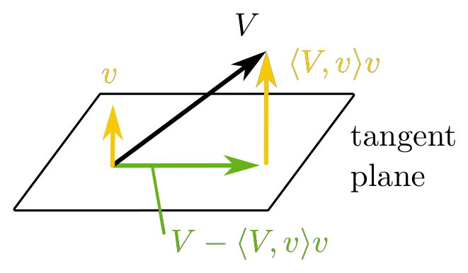
Let \(\Sigma\) be a regular hypersurface with Gauss map \(\nu\), and \(\gamma(t)\) be a smooth curve on \(\Sigma\). Given two vector fields \(X\) and \(Y\) on \(\Sigma\), we define the covariant derivative of \(X\) at \(p\in M\) along \(Y\) to be \[ \nabla_Y X(p) := (D_Y X(p))^\top = \left(D_Y X - \langle D_Y X, \nu\rangle\nu\right)(p). \] Here \((D_Y X(p))^\top\) represents the projection of \(D_Y X(p)\) onto the tangent space \(\Tp{p}\Sigma\).
Using the fact that \(\langle D_Y X, \nu\rangle = h(X,Y) = h_{ij}X^i Y^j\) and (3.11), we can derive the local expression for \(\nabla_Y X\): \[ \tag{3.12} \nabla_Y X = \underbrace{\sum_{i,j}\left(\pd{X^j}{u_i}\pdF{u_j} + X^j\pd{^2\mathbf{F}}{u_i\partial u_j}\right)Y^i}_{D_Y X} - \underbrace{\left(\sum_{i,j} h_{ij}X^i Y^j\right)\nu}_{\langle D_Y X,\nu\rangle\nu}. \]
Suppose \(X, \tilde{X}, Y\) and \(\tilde{Y}\) are vector fields and \(\phi\) is a smooth scalar function. One can verify that the following properties hold:
- \(\nabla_{\phi Y} X = \phi\nabla_Y X\)
- \(\nabla_Y(\phi X) = (\nabla_Y \phi)X + \phi\nabla_Y X\)
- \(\nabla_{Y+\tilde{Y}} X = \nabla_Y X + \nabla_{\tilde{Y}} X\)
- \(\nabla_Y(X+\tilde{X}) = \nabla_Y X + \nabla_Y\tilde{X}\)
For a scalar function \(\phi\), both \(\nabla_Y\phi\) and \(D_Y\phi\) represent the directional derivative of \(\phi\) along \(Y\) direction. Since they are scalars, so there is no such thing called “projection of a scalar onto the tangent plane”. We could use either \(\nabla_Y\phi\) or \(D_Y\phi\) for our convenience.
According to (3.11) and (3.12), given any vector fields \(X = X^i\pdF{u_i}\) and \(Y = Y^i\pdF{u_i}\), the second derivatives \(\pd{^2\mathbf{F}}{u_i\partial u_j}\) determine both \(D_Y X\) and \(\nabla_Y X\). We are going to express \(\pd{^2\mathbf{F}}{u_i\partial u_j}\) in terms of the tangent-normal basis \(\left\{\pdF{u_1},\ldots,\pdF{u_n},\nu\right\}\) of \(\mathbb{R}^{n+1}\). From (3.12), we have: \[ \pd{^2\mathbf{F}}{u_i\partial u_j} = D_{\pdF{u_j}}\pdF{u_i} = \nabla_{\pdF{u_j}}\pdF{u_i} + h_{ij}\nu. \] We denote the coefficients of the tangent vector \(\nabla_{\pdF{u_j}}\pdF{u_i}\) by the following Christoffel symbols: \[ \tag{3.13} \nabla_{\pdF{u_j}}\!\left(\pdF{u_i}\right) = \Gamma^k_{ij}\pdF{u_k}. \] The Christoffel symbols can be shown to depend only on the first fundamental form \(g\). We will use it to prove that Gauss curvature depends also only on \(g\) but not on \(h\).
In a local coordinate system \((u_1,\ldots,u_n)\), the Christoffel symbols \(\Gamma^k_{ij}\)’s can be locally expressed in terms of the first fundamental form as: \[ \tag{3.14} \Gamma^k_{ij} = \frac{1}{2}\,g^{kl}\left(\pd{g_{jl}}{u_i} + \pd{g_{il}}{u_j} - \pd{g_{ij}}{u_l}\right). \]
Recall that \(g_{ij} = \left\langle\pdF{u_i},\pdF{u_j}\right\rangle\). Differentiating with respect to \(u_l\): \[ \pd{g_{ij}}{u_l} = \left\langle\pd{^2\mathbf{F}}{u_l\partial u_i},\pdF{u_j}\right\rangle + \left\langle\pd{^2\mathbf{F}}{u_l\partial u_j},\pdF{u_i}\right\rangle. \] Using (3.13), i.e. \(\pd{^2\mathbf{F}}{u_l\partial u_i} = \Gamma^k_{li}\pdF{u_k}+h_{li}\nu\), we get: \[ \pd{g_{ij}}{u_l} = \Gamma^k_{li}g_{kj} + \Gamma^k_{lj}g_{ki}. \quad (*) \]
By cyclic permutation of indices \(\{i,j,l\}\) in (*): \[ \pd{g_{il}}{u_j} = \Gamma^k_{ij}g_{kl} + \Gamma^k_{jl}g_{ki}, \quad (**) \qquad \pd{g_{jl}}{u_i} = \Gamma^k_{ji}g_{kl} + \Gamma^k_{il}g_{kj}. \quad (***) \] Recall that \(\Gamma^k_{ij}=\Gamma^k_{ji}\) and \(h_{ij}=h_{ji}\). Considering \((**)+(***)-(*)\), we get: \[ \tag{3.15} \pd{g_{il}}{u_j} + \pd{g_{jl}}{u_i} - \pd{g_{ij}}{u_l} = 2\Gamma^k_{ij}g_{kl}. \]
Finally, multiplying \(g^{lq}\) on both sides of (3.15) and summing over all \(l\): \[ g^{lq}\left(\pd{g_{il}}{u_j}+\pd{g_{jl}}{u_i}-\pd{g_{ij}}{u_l}\right) = 2g^{lq}\Gamma^k_{ij}g_{kl} = 2\Gamma^k_{ij}\delta^q_k = 2\Gamma^q_{ij}. \] Relabelling \(q\) by \(k\) completes the proof of (3.14). \(\square\)