2.3 Transition Maps
One essential concept of regular surfaces is that we can locally parametrize a surface in several different ways. Take the sphere as an example, we can parametrize it as a graph \(z=f(x,y)\), or using stereographic parametrization. Suppose \(\bF(u,v)\) and \(\bG(s,t)\) are two regular parametrizations of the same surface, then on the overlap part of the images of \(\bF\) and \(\bG\), each \((u,v)\)-coordinates corresponds a unique \((s,t)\)-coordinates. We can then view \((u,v)\) as a function of \((s,t)\), and vice versa \((s,t)\) as a function of \((u,v)\). As the course is about differential geometry, it is crucial to know whether these functions are differentiable, or even \(C^\infty\). We are going to address this issue in this chapter.
Let \(M\subset\R^3\) be a regular surface, and \(\bF_\alpha(u_1,u_2):U_\alpha\to M\) and \(\bF_\beta(v_1,v_2):U_\beta\to M\) be two smooth local parametrizations of \(M\) with overlapping images, i.e. \(W:=\bF_\alpha(U_\alpha)\cap\bF_\beta(U_\beta)\neq\varnothing\). Under this set-up, it makes sense to define the maps \(\bF_\beta^{-1}\circ\bF_\alpha(u_1,u_2)\) and \(\bF_\alpha^{-1}\circ\bF_\beta(v_1,v_2)\). However, we need to shrink their domains so as to guarantee they are well-defined. Precisely:
\[(\bF_\beta^{-1}\circ\bF_\alpha):\bF_\alpha^{-1}(W)\to\bF_\beta^{-1}(W)\qquad(\bF_\alpha^{-1}\circ\bF_\beta):\bF_\beta^{-1}(W)\to\bF_\alpha^{-1}(W)\]
Note that \(\bF_\alpha^{-1}(W)\) and \(\bF_\beta^{-1}(W)\) are open subsets of \(U_\alpha\) and \(U_\beta\) respectively. The map \(\bF_\beta^{-1}\circ\bF_\alpha\) describes a relation between two sets of coordinates \((u_1,u_2)\) and \((v_1,v_2)\) of \(M\). In other words, one can regard \(\bF_\beta^{-1}\circ\bF_\alpha\) as a change-of-coordinates, or transition map and we can write \[\bF_\beta^{-1}\circ\bF_\alpha(u_1,u_2)=(v_1(u_1,u_2),\,v_2(u_1,u_2)).\]
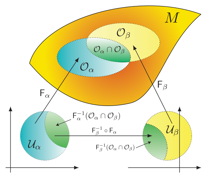
One goal of this chapter is to show that this transition map \(\bF_\beta^{-1}\circ\bF_\alpha\) is smooth provided that \(\bF_\alpha\) and \(\bF_\beta\) are two overlapping smooth local parametrizations. Before we present the proof, let us look at some examples of transition maps.
The \(xy\)-plane \(\Pi\) in \(\R^3\) is a regular surface which admits a global smooth parametrization \(\bF_\alpha(x,y)=(x,y,0):\R^2\to\Pi\). Another way to locally parametrize \(\Pi\) is by polar coordinates \(\bF_\beta:(0,\infty)\times(0,2\pi)\to\Pi\), \(\bF_\beta(r,\theta)=(r\cos\theta,r\sin\theta,0)\).
Readers should verify that they are smooth local parametrizations. The image of \(\bF_\alpha\) is the entire \(xy\)-plane \(\Pi\), whereas the image of \(\bF_\beta\) is the \(xy\)-plane with the origin and positive \(x\)-axis removed. The transition map \(\bF_\alpha^{-1}\circ\bF_\beta\) is given by \[\bF_\alpha^{-1}\circ\bF_\beta:(0,\infty)\times(0,2\pi)\to\R^2\setminus\{(x,0):x\ge 0\},\quad (r,\theta)\mapsto(r\cos\theta,r\sin\theta).\] To put it in a simpler form, we can say \((x(r,\theta),y(r,\theta))=(r\cos\theta,r\sin\theta)\). \(\square\)
Consider the stereographic parametrizations \(\bF_+\) and \(\bF_-\) in Example 2.5. Compute the transition maps \(\bF_+^{-1}\circ\bF_-\) and \(\bF_-^{-1}\circ\bF_+\). State the maximum possible domain for each map. Are they smooth on their domains?
The unit cylinder \(\Sigma^2\) in \(\R^3\) can be covered by two local parametrizations \(\bF:(0,2\pi)\times\R\to\Sigma^2\), \(\bF(\theta,z)=(\cos\theta,\sin\theta,z)\) and \(\widetilde{\bF}:(-\pi,\pi)\times\R\to\Sigma^2\), \(\widetilde{\bF}(\widetilde\theta,\widetilde z)=(\cos\widetilde\theta,\sin\widetilde\theta,\widetilde z)\). Compute the transition maps \(\bF^{-1}\circ\widetilde{\bF}\) and \(\widetilde{\bF}^{-1}\circ\bF\). State their maximum possible domains. Are they smooth on their domains?
The Möbius strip \(\Sigma^2\) in \(\R^3\) can be covered by two local parametrizations \(\bF:(-1,1)\times(0,2\pi)\to\Sigma^2\) and \(\widetilde{\bF}:(-1,1)\times(-\pi,\pi)\to\Sigma^2\) given by \[\bF(u,\theta)=\Big(\big(3+u\cos\tfrac{\theta}{2}\big)\cos\theta,\ \big(3+u\cos\tfrac{\theta}{2}\big)\sin\theta,\ u\sin\tfrac{\theta}{2}\Big),\] and \(\widetilde{\bF}\) given by the same formula in the tilded variables. Compute the transition maps, state their maximum possible domains and verify that they are smooth.
The proposition below shows that the transition maps between any pair of smooth local parametrizations are smooth:
Let \(M\subset\R^3\) be a regular surface, and \(\bF_\alpha(u_1,u_2):U_\alpha\to M\) and \(\bF_\beta(v_1,v_2):U_\beta\to M\) be two smooth local parametrizations of \(M\) with overlapping images, i.e. \(W:=\bF_\alpha(U_\alpha)\cap\bF_\beta(U_\beta)\neq\varnothing\). Then, the transition maps defined below are also smooth maps: \[(\bF_\beta^{-1}\circ\bF_\alpha):\bF_\alpha^{-1}(W)\to\bF_\beta^{-1}(W)\qquad(\bF_\alpha^{-1}\circ\bF_\beta):\bF_\beta^{-1}(W)\to\bF_\alpha^{-1}(W).\]
It suffices to show \(\bF_\beta^{-1}\circ\bF_\alpha\) is smooth as the other one \(\bF_\alpha^{-1}\circ\bF_\beta\) can be shown by symmetry. Furthermore, since differentiability is a local property, we may fix a point \(p\in W\subset M\) and show that \(\bF_\beta^{-1}\circ\bF_\alpha\) is smooth at the point \(\bF_\alpha^{-1}(p)\).
By condition (3) of smooth local parametrizations, we have \(\pd{\bF_\alpha}{u_1}(p)\times\pd{\bF_\alpha}{u_2}(p)\neq\mathbf{0}\). By straightforward computations, one can show that this cross product is given by \[\pd{\bF_\alpha}{u_1}\times\pd{\bF_\alpha}{u_2}=\left(\det\Jac{y,z}{u_1,u_2}(p),\ \det\Jac{z,x}{u_1,u_2}(p),\ \det\Jac{x,y}{u_1,u_2}(p)\right).\]
Hence, at least one of the determinants is non-zero. Without loss of generality, assume that \(\det\Jac{x,y}{u_1,u_2}(p)\neq 0\). Both \(\pd{\bF_\alpha}{u_1}(p)\times\pd{\bF_\alpha}{u_2}(p)\) and \(\pd{\bF_\beta}{v_1}(p)\times\pd{\bF_\beta}{v_2}(p)\) are normal vectors to the surface at \(p\). Given that the former has non-zero \(\hat{\mathbf{k}}\)-component, then so does the latter. Therefore, we have \(\det\Jac{x,y}{v_1,v_2}(p)\neq 0\).
Then we proceed as in the proof of Proposition 2.9. Define \(\pi(x,y,z)=(x,y)\), then \(\pi\circ\bF_\beta:U_\beta\to\R^2\), \((v_1,v_2)\mapsto(x(v_1,v_2),y(v_1,v_2))\) has non-zero Jacobian determinant \(\det\Jac{x,y}{v_1,v_2}\) at \(p\). Therefore, by the Inverse Function Theorem, \((\pi\circ\bF_\beta)^{-1}\) exists and is smooth near \(p\). Since \(\bF_\beta^{-1}\circ\bF_\alpha=(\pi\circ\bF_\beta)^{-1}\circ(\pi\circ\bF_\alpha)\), and all of \((\pi\circ\bF_\beta)^{-1},\pi\) and \(\bF_\alpha\) are smooth maps, their composition is also a smooth map. We have proved \(\bF_\beta^{-1}\circ\bF_\alpha\) is smooth near \(p\). Since \(p\) is arbitrary, \(\bF_\beta^{-1}\circ\bF_\alpha\) is in fact smooth on the domain \(\bF_\alpha^{-1}(W)\). \(\square\)
Rewrite the proof of Proposition 2.12, mutatis mutandis, by assuming \(\det\Jac{y,z}{u_1,u_2}(p)\neq 0\) instead.
Chain rule for tangent vectors
One consequence of Proposition 2.12 is that it allows us to apply the chain rule to convert a tangent vector from one basis to another. Recall from linear algebra that given two bases \(\{\mathbf{x}_1,\mathbf{x}_2\}\) and \(\{\mathbf{y}_1,\mathbf{y}_2\}\) of \(\R^2\), then to convert a vector \(\mathbf{v}=a\mathbf{x}_1+b\mathbf{x}_2\) using the basis \(\{\mathbf{y}_1,\mathbf{y}_2\}\) one then needs to solve a system of equations \(\gamma\mathbf{y}_1+\delta\mathbf{y}_2=\mathbf{v}\) for \(\gamma\) and \(\delta\). However, given two local parametrizations \(\bF(u_1,u_2)\) and \(\bG(v_1,v_2)\), then to convert a tangent vector \(a\,\pdF{u_1}+b\,\pdF{u_2}\) using the basis \(\big\{\pdG{v_1},\pdG{v_2}\big\}\), one can use the chain rule by regarding \(\bF\) as \(\bG\circ(\bG^{-1}\circ\bF)\). Then, we have
\[\begin{aligned}\pdF{u_1}&=\pd{}{u_1}\,\bG\circ(\bG^{-1}\circ\bF)=\pdG{v_1}\pd{v_1}{u_1}+\pdG{v_2}\pd{v_2}{u_1},\\[4pt]\pdF{u_2}&=\pdG{v_1}\pd{v_1}{u_2}+\pdG{v_2}\pd{v_2}{u_2}.\end{aligned}\]
Therefore, so long as we can express \((v_1,v_2)\) as a differentiable function of \((u_1,u_2)\), we can freely convert tangent vectors from one basis \(\big\{\pdF{u_1},\pdF{u_2}\big\}\) to another \(\big\{\pdG{v_1},\pdG{v_2}\big\}\).
Consider the two parametrizations of the \(xy\)-plane in Example 2.11. We have two coordinate systems \(\bF_\alpha(x,y)=(x,y,0)\) and \(\bF_\beta(r,\theta)=(r\cos\theta,r\sin\theta,0)\). To convert one tangent vector basis to another one, we do use the chain rule as discussed above:
\[\begin{aligned}\pd{\bF_\beta}{r}&=\pd{\bF_\alpha}{x}\pd{x}{r}+\pd{\bF_\alpha}{y}\pd{y}{r}=(\cos\theta)\pd{\bF_\alpha}{x}+(\sin\theta)\pd{\bF_\alpha}{y}\\[4pt]&=\frac{x}{\sqrt{x^2+y^2}}\pd{\bF_\alpha}{x}+\frac{y}{\sqrt{x^2+y^2}}\pd{\bF_\alpha}{y}.\end{aligned}\]
Express \(\pd{\bF_\beta}{\theta}\) in the above example as a linear combination of \(\pd{\bF_\alpha}{x}\) and \(\pd{\bF_\alpha}{y}\).
Given two parametrizations \(\bF(u_1,u_2)\) and \(\bG(v_1,v_2)\), verify that \[\begin{bmatrix}\pdF{u_1}&\pdF{u_2}\end{bmatrix}=\Jac{u_1,u_2}{v_1,v_2}\begin{bmatrix}\pdG{v_1}&\pdG{v_2}\end{bmatrix}.\]
Parametrization-independence of surface area
Let’s also see some deeper use of the change-of-variable formula. The area element of a regular surface, parametrized by \(\bF(u_1,u_2)\), is given by \[dS=\left|\pdF{u_1}\times\pdF{u_2}\right|du_1\,du_2.\] As we recall in multivariable calculus, the surface integral of a parametrized surface \(\bF(u_1,u_2)\) over the region \(R\subset\R^2\) is defined as \[\int_{\bF(R)} f\,dS=\int_R f(\bF(u_1,u_2))\left|\pdF{u_1}\times\pdF{u_2}\right|du_1\,du_2.\]
When the function \(f\) is identically equal to \(1\), the above integral represents the surface area of \(\bF(R)\). We should expect that the surface area should be independent of the choice of parametrization. Let’s verify this is the case. Suppose \(\bG(v_1,v_2)\) is another parametrization of the surface. We need to check that \[\left|\pdF{u_1}\times\pdF{u_2}\right|du_1\,du_2=\left|\pdG{v_1}\times\pdG{v_2}\right|dv_1\,dv_2.\]
Using the chain rule, we have \[\pdG{v_1}=\pdF{u_1}\pd{u_1}{v_1}+\pdF{u_2}\pd{u_2}{v_1},\qquad\pdG{v_2}=\pdF{u_1}\pd{u_1}{v_2}+\pdF{u_2}\pd{u_2}{v_2}.\] In fact, it is easier to work with summation notations: \(\displaystyle \pdG{v_j}=\sum_{i=1}^{2}\pdF{u_i}\pd{u_i}{v_j}.\) Then, we have
\[\begin{aligned}\pdG{v_1}\times\pdG{v_2}&=\left(\sum_k \pd{u_k}{v_1}\pdF{u_k}\right)\times\left(\sum_l \pd{u_l}{v_2}\pdF{u_l}\right)\\[4pt]&=\sum_{k,l}\left(\pd{u_k}{v_1}\pd{u_l}{v_2}\right)\pdF{u_k}\times\pdF{u_l}.\end{aligned}\]
Although the last line is a sum of four terms, two of them – when \((k,l)=(1,1)\) or \((2,2)\) – are zero by the property of cross product. Therefore, we have \[\begin{aligned}\pdG{v_1}\times\pdG{v_2}&=\left(\pd{u_1}{v_1}\pd{u_2}{v_2}\right)\pdF{u_1}\times\pdF{u_2}\\[4pt]&\quad+\left(\pd{u_2}{v_1}\pd{u_1}{v_2}\right)\pdF{u_2}\times\pdF{u_1}.\end{aligned}\]
Recall that cross product is skew-symmetric, so we have \[\pdG{v_1}\times\pdG{v_2}=\left(\pd{u_1}{v_1}\pd{u_2}{v_2}-\pd{u_2}{v_1}\pd{u_1}{v_2}\right)\pdF{u_1}\times\pdF{u_2}.\]
The scalar term is in fact the determinant of the Jacobian matrix \[\Jac{u_1,u_2}{v_1,v_2}=\begin{bmatrix}\pd{u_1}{v_1}&\pd{u_1}{v_2}\\[2pt]\pd{u_2}{v_1}&\pd{u_2}{v_2}\end{bmatrix}.\] Hence, we conclude that \[\left|\pdG{v_1}\times\pdG{v_2}\right|=\left|\det\Jac{u_1,u_2}{v_1,v_2}\right|\left|\pdF{u_1}\times\pdF{u_2}\right|.\]
Coincidentally, the change-of-variable formula between \(du_1\,du_2\) and \(dv_1\,dv_2\) is given by \(\displaystyle dv_1\,dv_2=\left|\det\Jac{v_1,v_2}{u_1,u_2}\right|du_1\,du_2.\) Combining the previous result, we have
\[\begin{aligned}\left|\pdG{v_1}\times\pdG{v_2}\right|dv_1\,dv_2&=\left|\pdF{u_1}\times\pdF{u_2}\right|\left|\det\Jac{u_1,u_2}{v_1,v_2}\right|\left|\det\Jac{v_1,v_2}{u_1,u_2}\right|du_1\,du_2\\[4pt]&=\left|\pdF{u_1}\times\pdF{u_2}\right|\left|\det\!\left(\Jac{u_1,u_2}{v_1,v_2}\Jac{v_1,v_2}{u_1,u_2}\right)\right|du_1\,du_2.\end{aligned}\]
This completes the proof by observing that the product matrix \(\Jac{u_1,u_2}{v_1,v_2}\Jac{v_1,v_2}{u_1,u_2}\) is the identity matrix whose determinant is \(1\).
Both \(\pdF{u_1}\times\pdF{u_2}\) and \(\pdG{v_1}\times\pdG{v_2}\) are normal vectors to the regular surface. Under what condition are they pointing at the same direction?
In differential geometry, it is often the case that we define geometric quantities (such as curvature) using local parametrizations. It is then essential to verify that these quantities are independent of local parametrizations.
In general relativity in physics, one postulate is that physical laws are independent of observers whose inertial frames are different. It is known as the equivalence principle. In mathematical terms, different inertial frames basically means different local parametrizations (or coordinates). Checking that a physical law is independent of inertial frames is basically like verifying that the law is independent of the choice of local parametrizations. Differential geometry and physics are from the same family!